Matrix Decomposition Decoded

This article covers matrix decomposition, as well as the underlying concepts of eigenvalues (lambdas) and eigenvectors, as well as discusses the purpose behind using matrix and vectors in linear algebra.

comments

By Tanveer Sayyed, Data Science Enthusiast

To understand matrix decomposition we’ll have to first understand eigenvalues(referred to as lambdas here on) and eigenvectors. And even before comprehending the intuition behind lambdas and eigenvectors we’ll first need to uncover the purpose behind using matrix and vectors in linear algebra.

So what is the purpose of a matrix and a vector in linear algebra?

In machine learning we are usually concerned with matrices which have features as their columns. We have thus innately made matrices sacrosanct in our minds. Now this might come as a surprise because — the purpose of a matrix is to “act” on (input) vectors to give (output) vectors! Recall the equation of linear regression using linear algebra:

 (X^T . X)^-1 . X^T   .       y         ------>  coefficients
[---m-a-t-r-i-x----]  . [input vector]  ------> [output vector]

The correct way to read this is — we ‘apply’ the matrix to a vector(y) to get the output vector(coefficients). Or in other words — the matrix ‘transforms/distorts’ the input vector to become the output vector. In goes a vector, gets transformed/distorted by a matrix, and out comes another vector. This is just like a function in calculus: in goes a number x(say 3) and outcomes a number f(x)[say 27, if f(x) = x³].

The intuition behind lambdas and eigenvectors

Since the purpose of matrices are now clear, defining eigenvectors would be easy. If we find that, the input vector which goes in and the output vector which comes out, are still parallel to each other, only then that vector is called eigenvector. Which means they have sustained the distortion or are not affected by it. “Parallel” refers to either one of the two:


     ------------>                          ------------>
     ------------>                          <------------
          1.                                     2.

At school we were taught that Force is a vector. It has a direction as well as a magnitude. The same way think of eigenvectors as the direction of the distortion and lambdas as the magnitude of distortion in ‘that’ direction. Thus a matrix is decomposed/factorized(just like 6= 3*2) into a vector and its magnitude which can be written as a product of both:


A.x = λ x 
 where,
 …… A is a square matrix,
 …… x is eigenvector of A 
 …… λ is the scalar eigenvalue

This is called eigen-decomposition. But how do we find eigenvectors? From the λs! Here is how:


A.x - λx = 0    …. (rearranging above equation)
(A -  λI) . x = 0 …. (eq.1)Now x is a non-zero vector. 
In matrices, if we want the product to be equal to zero, 
then the term (A - λI) must be singular! That is, 
the determinant of this whole term must be = 0. 
Hence,
|A - λI| = 0 ….. (eq.2) Solve eq.2 and 
substitute ‘each’ value of λ in eq.1 to get 
the corresponding eigenvector for that λ.

What was important was knowing and understanding these steps so we’ll not do this manually because a function already exists in numpy library. (And we’ll be using this code to display and re-scale the eigenvectors). An example:

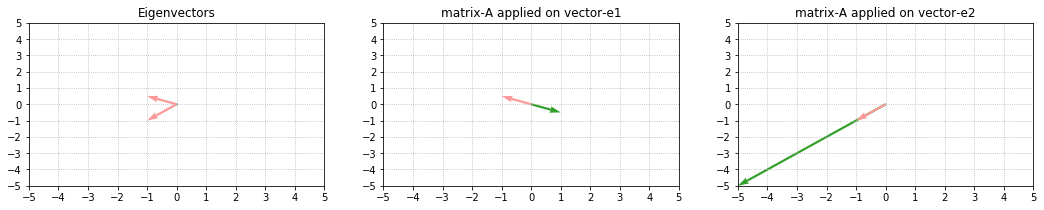
Eigenvectors e1 = [-1, 0.5] and e2 = [-1, -1] are in PINK while the output vector is in GREEN.

Note the effect of lambdas [-1, 5]. The lambdas are responsible for the scaling(change in size) of the eigenvectors. λ1 is negative, hence we observe negative transformation — output vector moves opposite to e1 and gets scaled 1 times length of e1. While λ2 is positive and hence we observe positive transformation — output vector moves in the same direction as e2 and gets scaled 5 times length of e2.

Now before we move to applications of the eigenvectors and lambdas lets first get their properties into place:

1. We can only find eigenvectors and lambdas of a square matrix.
2. If A has the shape(n,n) then there would be at-most n no. of independent lambdas and their corresponding eigenvectors.


-------------->-------------->-------------------------->------
            (2,2)          (4,4)                      (8,8)
Take the line above. We can observe 3 eigenvectors, but they are not 
independent as they are just multiples of each other and are part of the same line x = y.

3. The sum of lambdas = trace(sum of diagonals) of the matrix.
4. The product of lambdas = determinant of the matrix-A.
5. For a triangular matrix the lambdas are the diagonal values.
6. Repeated lambdas are a source of trouble. For every one lambda repeated we will have one less independent eigenvector.

7. The more symmetric the matrix the better. Symmetric means A = transpose(A). Symmetric matrices produce “real” lambdas. As we start moving away from symmetric to asymmetric matrices the lambdas start becoming complex numbers(a +ib) and hence eigenvectors start mapping to the imaginary space instead of the real space. This happens despite every element of matrix-A being a real number as we see in the adjacent code.

Applications of eigenvectors and lambdas

Firstly, let us be clear that eigenvalues(lambdas) are not linear. Which means if x, α and y, β are eigenvalues and lambdas of matrices A, B respectively then:

A . B ≠ αβ (x . y), and, A + B ≠ αx + βy.

But they do come handy when it comes to calculating powers of matrices i.e. finding A²⁰ or B⁵⁰⁰. If A, B are small matrices it might be possible to calculate the result on our machines. But imagine a huge matrix with lots of features as columns, would it be feasible then? Would we punch-in B 500 times or run a loop 500 times? No, because matrix multiplication are computationally exhaustive. So let’s understand how “the Eigens” come to the rescue by discussing the second way of factorization/decomposition of the same matrix. And that is derived from the following equation:


S^-1 . A . S = Λ …. (eq.3)
where,
      S* is eigenvector matrix (each eigenvector of A is a column in matrix-S)
      A is our square matrix
      Λ (capital lambda) is a diagonal matrix of all lambda values*[For S to be invertible, all eigenvectors must be independent (the above stated property-2 must be satisfied). And by the way, very few matrices fulfill it].
Now, let's get our matrix from eq.3:
1. Left multiplication by S     --> (S.S^-1).A.S = S.Λ
                                --> A.S = S.Λ
2. Right multiplication by S^-1 --> A.S.(S^-1) = S.Λ.(S^-1)
                                --> A = S.Λ.S^-1
The matrix A has thus been factorized into three terms: S and Λ and S^-1.
Now 12² can also be calculated as squares of its prime factors viz 3² * 2² * 2². 
Similarly lets also do for A²:
A² = A . A 
   = (S . Λ . S^-1).(S . Λ . S^-1)
   =  S . Λ . (S^-1 . S) . Λ . S^-1
   =  S . Λ . Λ . S^-1
A² =  S . Λ². S^-1
Generalizing as:
A^K = S . Λ^K. S^-1

Now see how convenient it is to calculate large powers via factorization.

Now let’s dive a little more deeper into why exactly does this happen. Take another example:

Observe the eigenvectors of F¹ and F⁵. They remain undistorted and keep pointing in the same direction. Thus powers of a matrix has absolutely no effect on eigenvectors! But observe both the lambdas when degree is changed from 1 to 5; λ1 is increasing(1.618 to 11.09) much more rapidly than λ2 is decreasing(-0.618 to -0.09). Thus the effect of λ2 almost negligible. This shows that overall the matrix is an increasing one, which can be validated from its values in F⁵[5,3,3,2].

Since we know that matrix multiplications are computationally exhaustive then for any square matrix, if it’s each |λ|is < 0 then we know that the matrix is a stable matrix and if each |λ|is >0 then the matrix is blowing up and is an unstable matrix so its better not to move ahead.

The above example is actually the Fibonacci matrix where the matrix F increases/gets scaled approx 1.6180399 times each time it multiplies itself! Let’s confirm this:


0, 1, 1, 2, 3, 5, 8, 13, 21, 34.... is the Fibonacci Series
5 * 1.6180399 ≈ 8
8 * 1.6180399 ≈ 13
13 * 1.6180399 ≈ 21

And that number is the value of lambda itself … isn’t that amazing!!!
The beauty of lambdas(eigenvalues) is that despite being very few in number they can open-up hidden secrets about the properties of that matrix/the transforming function.

Another application of “the Eigens” is of-course, principle component analysis — PCA !

Why PCA?

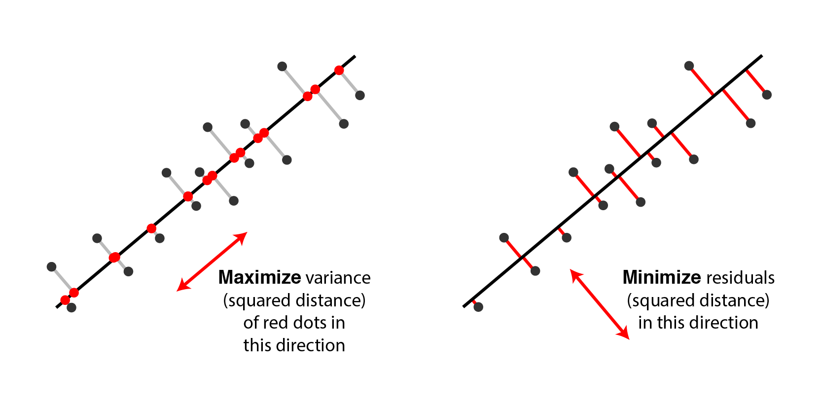
PCA is used for feature extraction/dimensionality reduction, which refers to the method of reducing the known variables of the data, by projection, into lesser number of variables holding the “almost” the same amount of information. There are two equivalent ways to interpret PCA:

(i) minimize the projection error,
(ii) maximize the variance of the projection.

Here it is extremely important to note that both the above statements are actually two sides of the same coin, so minimizing one is equivalent to maximizing the second.

Credits

What is the need for projection?

We need it because when there are say 1000 features, then, we have 1000 unknown variables. It turns out we need 1000 simultaneous equations to solve for all the variables! But “what if” no solutions exists to the problem at hand?...! For example just take a case of 2-variables:

a + b = 2

a + 2b = 2 …. ?

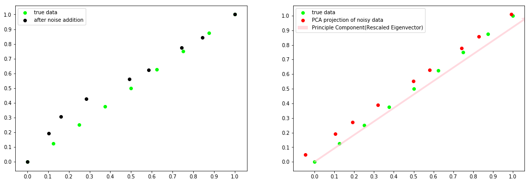
What PCA does is, it finds the closest approximation to the problem at hand such that certain properties of the initial data are preserved(in other words noise is reduced). Projection thus helps separate noise from the data(code illustration below). This is done by minimizing the least square projection error, which gives the best possible solution.

Is minimizing projection error same as minimizing least square error in linear regression?

Nope. Here is how and why:

Credits: Andrew Ng

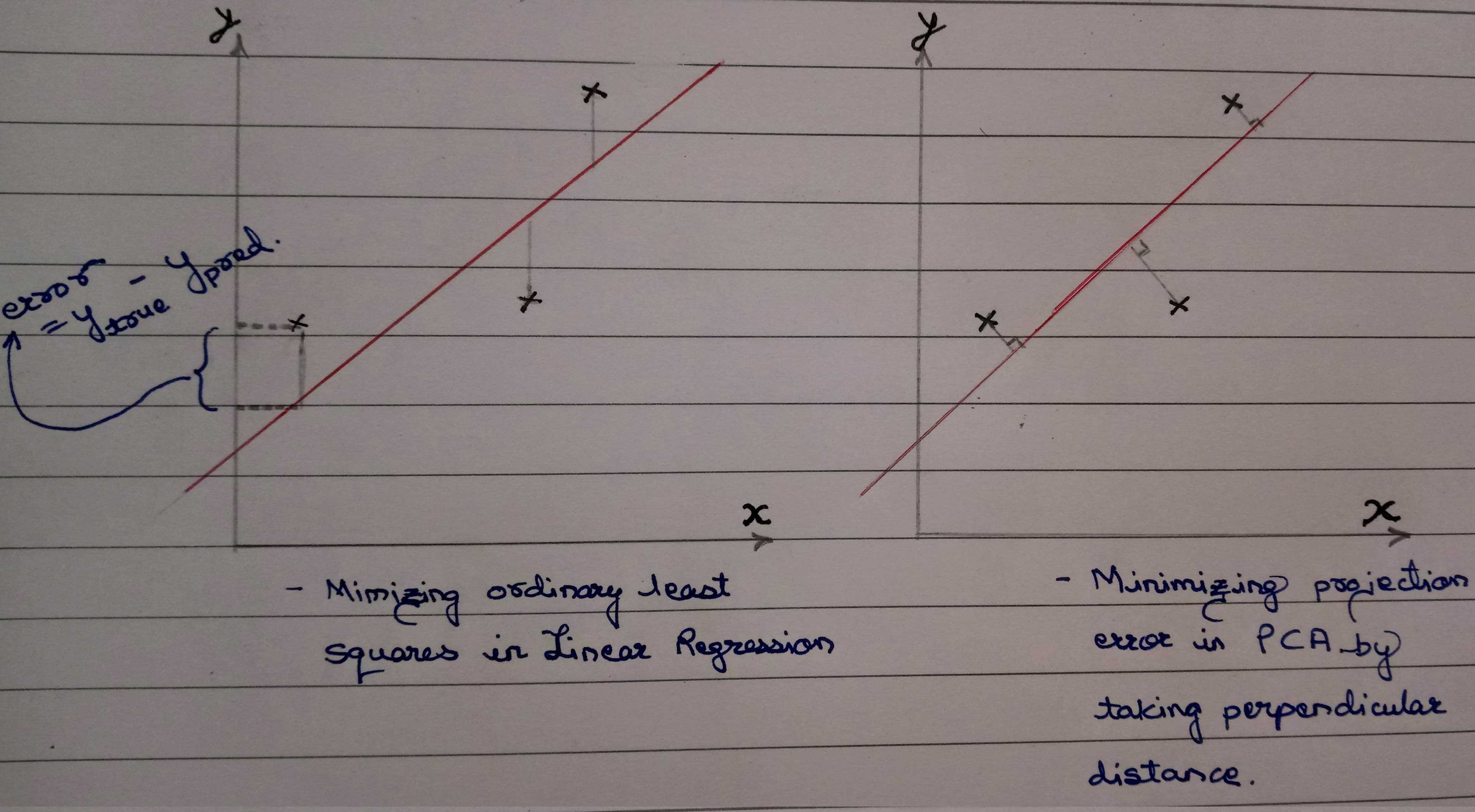
This diagram also gives a hint as to why PCA can also be used for unsupervised learning!

But where do “the Eigens” pitch in?

For that we’ll have to make ourselves aware of the steps of PCA:

Since PCA is sensitive to scaling, lets normalize/standardize out matrix-A first. M = mean(A) and then, C = A − M.
The next step is to remember that for best results i.e. to make use of “the Eigens” we need a square matrix and which is symmetrical(property-7 above). So which matrix satisfies both the conditions? Ummm… Ahaan! — the covariance matrix! So we do: V = cov(C)
As we now have what we want, lets just quickly decompose it.
lambdas, eigenvectors = np.linalg.eig(V )
The lambdas are then sorted in descending order. Their corresponding eigenvectors now represent the components of the reduced subspace. In the reduced subspace these components (eigenvectors) have now become our new axes, and we know that axes are always orthogonal to one another. (This can only happen when each component in PCA is an independent eigenvector). The combinations of these axes produce the projected data.(Click this link to get a better understanding. Make each component point directly at you. You’ll see that the first component has captured the highest variance followed by second and then the third)
Select k lambdas to retain maximum explained variance. The amount of variance captured by k number of lambdas is called explained variance.

What was important was knowing and understanding these steps so we’ll not do this manually because a function already exists in the sklearn library. For simplicity we will reduce a 2-dimenstional data to 1-dimensional data while observing the effect of noise during the process. Here is the code:

Note the projections are exactly parallel to the principle component. The near uniform closeness of the red and green dots (as compared to black and green dots) depicts that noise has been reduced to a good extent.

(If you identify anything wrong/incorrect, please do respond. Criticism is welcomed).

References:
https://www.youtube.com/playlist?list=PLE7DDD91010BC51F8(Prof. Gilbert Strang, Stanford University. Most of my content comes from here.)

A Gentle Introduction to Singular-Value Decomposition (SVD) for Machine Learning

https://www.youtube.com/watch?v=vs2sRvSzA3o (probably the best visual representation of eigenvalues and eigenvectors)

https://hadrienj.github.io/posts/Deep-Learning-Book-Series-Introduction/ (the code to visualize vectors)

https://en.wikipedia.org/wiki/Singular_value_decomposition

Everything you did and didn't know about PCA · Its Neuronal

Illustration of principal component analysis (PCA)

https://stats.stackexchange.com/questions/2691/making-sense-of-principal-component-analysis-eigenvectors-eigenvalues (superb thread)

Practical Guide to Principal Component Analysis (PCA) in R & Python

In Depth: Principal Component Analysis

https://medium.com/@zhang_yang/python-code-examples-of-pca-v-s-svd-4e9861db0a71