The Ultimate Scikit-Learn Machine Learning Cheatsheet

By Andre Ye, Cofounder at Critiq, Editor & Top Writer at Medium.

Source: Pixabay.

There are several areas of data mining and machine learning that will be covered in this cheat-sheet:

• Predictive Modelling. Regression and classification algorithms for supervised learning (prediction), metrics for evaluating model performance.
• Methods to group data without a label into clusters: K-Means, selecting cluster numbers based objective metrics.
• Dimensionality Reduction. Methods to reduce the dimensionality of data and attributes of those methods: PCA and LDA.
• Feature Importance. Methods to find the most important feature in a dataset: permutation importance, SHAP values, Partial Dependence Plots.
• Data Transformation. Methods to transform the data for greater predictive power, for easier analysis, or to uncover hidden relationships and patterns: standardization, normalization, box-cox transformations.

All images were created by the author unless explicitly stated otherwise.

Predictive Modelling

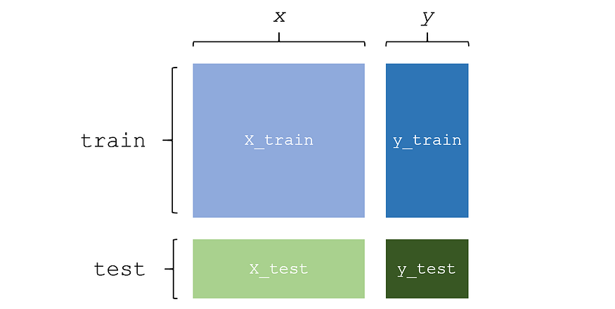
Train-test-split is an important part of testing how well a model performs by training it on designated training data and testing it on designated testing data. This way, the model’s ability to generalize to new data can be measured. In sklearn, both lists, pandas DataFrames, or NumPy arrays are accepted in X and y parameters.

from sklearn.model_selection import train_test_split
X_train,X_test,y_train,y_test = train_test_split(X,y,test_size=0.3)

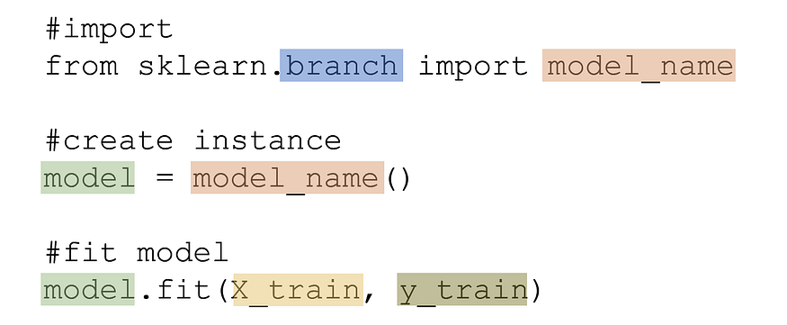
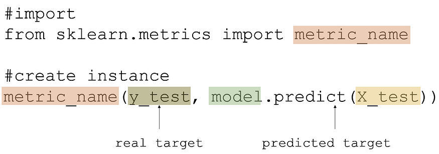
Training a standard supervised learning model takes the form of an import, the creation of an instance, and the fitting of the model.

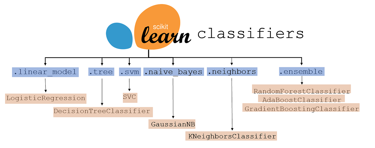
sklearn classifier models are listed below, with the branch highlighted in blue and the model name in orange.

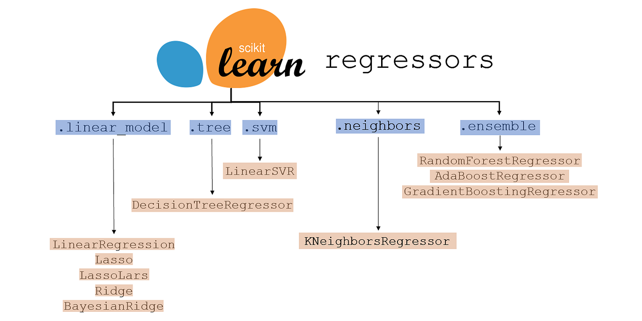
sklearn regressor models are listed below, with the branch highlighted in blue and the model name in orange.

Evaluating model performance is done with train-test data in this form:

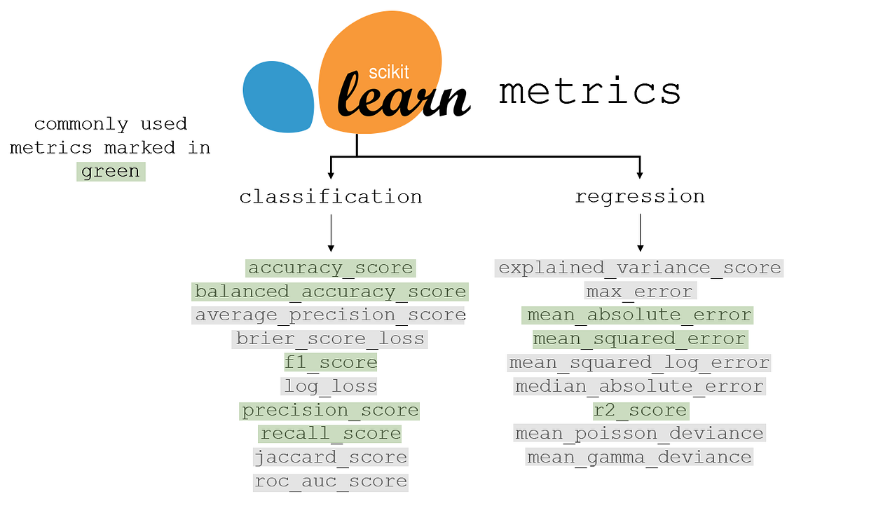
sklearn metrics for classification and regression are listed below, with the most commonly used metric marked in green. Many of the grey metrics are more appropriate than the green-marked ones in certain contexts. Each has its own advantages and disadvantages, balancing priority comparisons, interpretability, and other factors.

Clustering

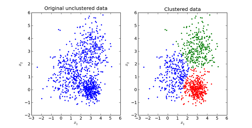
Before clustering, the data needs to be standardized (information for this can be found in the Data Transformation section). Clustering is the process of creating clusters based on point distances.

Source. Image free to share.

Training and creating a K-Means clustering model creates a model that can cluster and retrieve information about the clustered data.

from sklearn.cluster import KMeans
model = KMeans(n_clusters = number_of_clusters)
model.fit(X)

Accessing the labels of each of the data points in the data can be done with:

model.labels_

Similarly, the label of each data point can be stored in a column of the data with:

data['Label'] = model.labels_

Accessing the cluster label of new data can be done with the following command. The new_data can be in the form of an array, a list, or a DataFrame.

data.predict(new_data)

Accessing the cluster centers of each cluster is returned in the form of a two-dimensional array with:

data.cluster_centers_

To find the optimal number of clusters, use the silhouette score, which is a metric of how well a certain number of clusters fits the data. For each number of clusters within a predefined range, a K-Means clustering algorithm is trained, and its silhouette score is saved to a list (scores). data is the x that the model is trained on.

from sklearn.metrics import silhouette_score
scores = []
for cluster_num in range(lower_bound, upper_bound):
     model = KMeans(n_clusters=cluster_num)
     model.fit(data)
     score = silhouette_score(data, model.predict(data))

After the scores are saved to the list scores, they can be graphed out or computationally searched for to find the highest one.

Dimensionality Reduction

Dimensionality reduction is the process of expressing high-dimensional data in a reduced number of dimensions such that each one contains the most amount of information. Dimensionality reduction may be used for visualization of high-dimensional data or to speed up machine learning models by removing low-information or correlated features.

Principal Component Analysis, or PCA, is a popular method of reducing the dimensionality of data by drawing several orthogonal (perpendicular) vectors in the feature space to represent the reduced number of dimensions. The variable number represents the number of dimensions the reduced data will have. In the case of visualization, for example, it would be two dimensions.

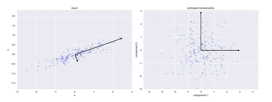
Visual demonstration of how PCA works. Source.

Fitting the PCA Model: The .fit_transform function automatically fits the model to the data and transforms it into a reduced number of dimensions.

from sklearn.decomposition import PCA
model = PCA(n_components=number)
data = model.fit_transform(data)

Explained Variance Ratio: Calling model.explained_variance_ratio_ will yield a list where each item corresponds to that dimension’s “explained variance ratio,” which essentially means the percent of the information in the original data represented by that dimension. The sum of the explained variance ratios is the total percent of information retained in the reduced dimensionality data.

PCA Feature Weights: In PCA, each newly creates feature is a linear combination of the former data’s features. These linear weights can be accessed with model.components_, and are a good indicator for feature importance (a higher linear weight indicates more information represented in that feature).

Linear Discriminant Analysis (LDA, not to be commonly confused with Latent Dirichlet Allocation) is another method of dimensionality reduction. The primary difference between LDA and PCA is that LDA is a supervised algorithm, meaning it takes into account both x and y. Principal Component Analysis only considers x and is hence an unsupervised algorithm.

PCA attempts to maintain the structure (variance) of the data purely based on distances between points, whereas LDA prioritizes clean separation of classes.

from sklearn.decomposition import LatentDirichletAllocation
lda = LatentDirichletAllocation(n_components = number)
transformed = lda.fit_transform(X, y)

Feature Importance

Feature Importance is the process of finding the most important feature to a target. Through PCA, the feature that contains the most information can be found, but feature importance concerns a feature’s impact on the target. A change in an ‘important’ feature will have a large effect on the y-variable, whereas a change in an ‘unimportant’ feature will have little to no effect on the y-variable.

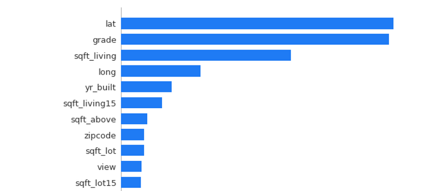
Permutation Importance is a method to evaluate how important a feature is. Several models are trained, each missing one column. The corresponding decrease in model accuracy as a result of the lack of data represents how important the column is to a model’s predictive power. The eli5 library is used for Permutation Importance.

import eli5
from eli5.sklearn import PermutationImportance
model = PermutationImportance(model)
model.fit(X,y)
eli5.show_weights(model, feature_names = X.columns.tolist())

In the data that this Permutation Importance model was trained on, the column lat has the largest impact on the target variable (in this case, the house price). Permutation Importance is the best feature to use when deciding which to remove (correlated or redundant features that actually confuse the model, marked by negative permutation importance values) in models for best predictive performance.

SHAP is another method of evaluating feature importance, borrowing from game theory principles in Blackjack to estimate how much value a player can contribute. Unlike permutation importance, SHapley Addative ExPlanations use a more formulaic and calculation-based method towards evaluating feature importance. SHAP requires a tree-based model (Decision Tree, Random Forest) and accommodates both regression and classification.

import shap
explainer = shap.TreeExplainer(model)
shap_values = explainer.shap_values(X)
shap.summary_plot(shap_values, X, plot_type="bar")

PD(P) Plots, or partial dependence plots, are a staple in data mining and analysis, showing how certain values of one feature influence a change in the target variable. Imports required include pdpbox for the dependence plots and matplotlib to display the plots.

from pdpbox import pdp, info_plots
import matplotlib.pyplot as plt

Isolated PDPs: the following code displays the partial dependence plot, where feat_name is the feature within X that will be isolated and compared to the target variable. The second line of code saves the data, whereas the third constructs the canvas to display the plot.

feat_name = 'sqft_living'
pdp_dist = pdp.pdp_isolate(model=model, 
                           dataset=X, 
                           model_features=X.columns,
                           feature=feat_name)
pdp.pdp_plot(pdp_dist, feat_name)
plt.show()

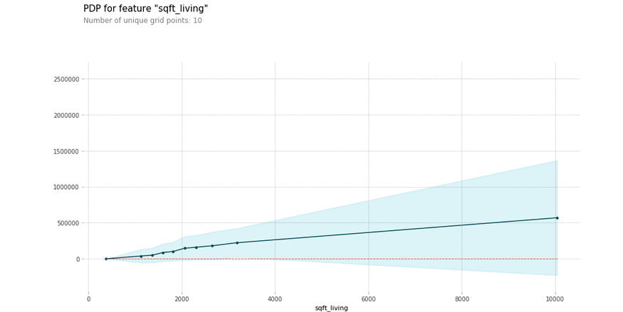
The partial dependence plot shows the effect of certain values and changes in the number of square feet of living space on the price of a house. Shaded areas represent confidence intervals.

Contour PDPs: Partial dependence plots can also take the form of contour plots, which compare not one isolated variable but the relationship between two isolated variables. The two features that are to be compared are stored in a variable compared_features.

compared_features = ['sqft_living', 'grade']
inter = pdp.pdp_interact(model=model, 
                          dataset=X, 
                          model_features=X.columns, 
                          features=compared_features)
pdp.pdp_interact_plot(pdp_interact_out=inter,
                      feature_names=compared_features),
                      plot_type='contour')
plt.show()

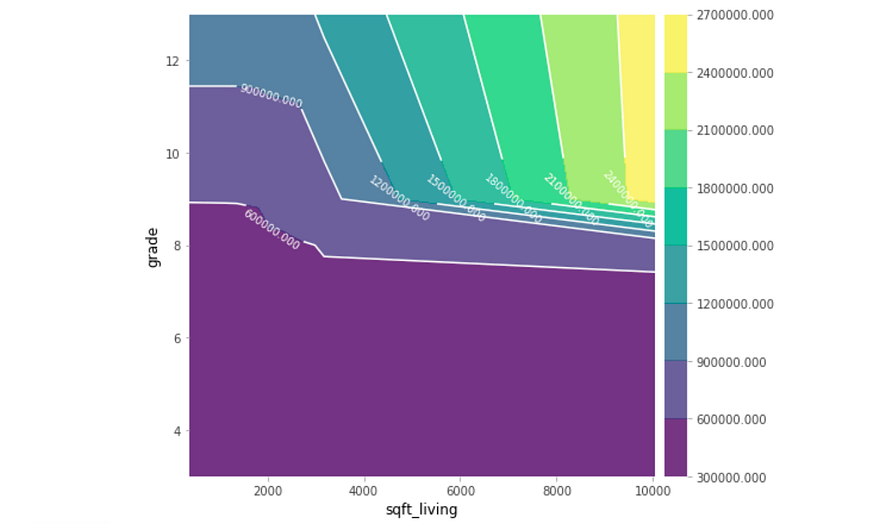
The relationship between the two features shows the corresponding price when only considering these two features. Partial dependence plots are chock-full of data analysis and findings, but be conscious of large confidence intervals.

Data Transformation

Standardizing or scaling is the process of ‘reshaping’ the data such that it contains the same information but has a mean of 0 and a variance of 1. By scaling the data, the mathematical nature of algorithms can usually handle data better.

from sklearn.preprocessing import StandardScaler
scaler = StandardScaler()
scaler.fit(data)
transformed_data = scaler.transform(data)

The transformed_data is standardized and can be used for many distance-based algorithms such as Support Vector Machine and K-Nearest Neighbors. The results of algorithms that use standardized data need to be ‘de-standardized’ so they can be properly interpreted. .inverse_transform() can be used to perform the opposite of standard transforms.

data = scaler.inverse_transform(output_data)

Normalizing data puts it on a 0 to 1 scale, something that, similar to standardized data, makes the data mathematically easier to use for the model.

from sklearn.preprocessing import Normalizer
normalize = Normalizer()
transformed_data = normalize.fit_transform(data)

While normalizing doesn’t transform the shape of the data as standardizing does, it restricts the boundaries of the data. Whether to normalize or standardize data depends on the algorithm and the context.

Box-cox transformations involve raising the data to various powers to transform it. Box-cox transformations can normalize data, make it more linear, or decrease the complexity. These transformations don’t only involve raising the data to powers but also fractional powers (square rooting) and logarithms.

For instance, consider data points situated along the function g(x). By applying the logarithm box-cox transformation, the data can be easily modelled with linear regression.

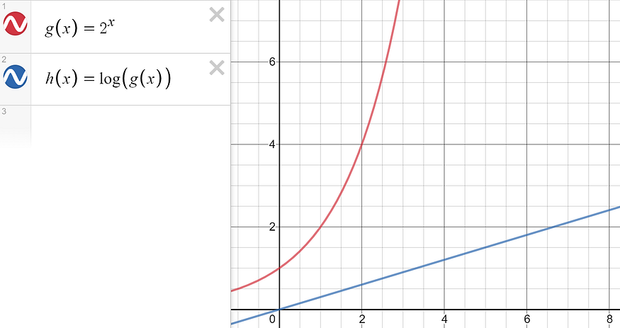
Created with Desmos.

sklearn automatically determines the best series of box-cox transformations to apply to the data to make it better resemble a normal distribution.

from sklearn.preprocessing import PowerTransformer
transformer = PowerTransformer(method='box-cox')
transformed_data = transformer.fit_transform(data)

Because of the nature of box-cox transformation square-rooting, box-cox transformed data must be strictly positive (normalizing the data beforehand can take care of this). For data with negative data points as well as positive ones, set method = ‘yeo-johnson’ for a similar approach to making the data more closely resemble a bell curve.

Original. Reposted with permission.

Related:

• 10 Things You Didn’t Know About Scikit-Learn
• How to Extend Scikit-learn and Bring Sanity to Your Machine Learning Workflow
• Machine Learning Cheat Sheets