How to Use Kafka Connect to Create an Open Source Data Pipeline for Processing Real-Time Data
This article shows you how to create a real-time data pipeline using only pure open source technologies. These include Kafka Connect, Apache Kafka, Kibana and more.
By Paul Brebner, Technology Evangelist at Instaclustr
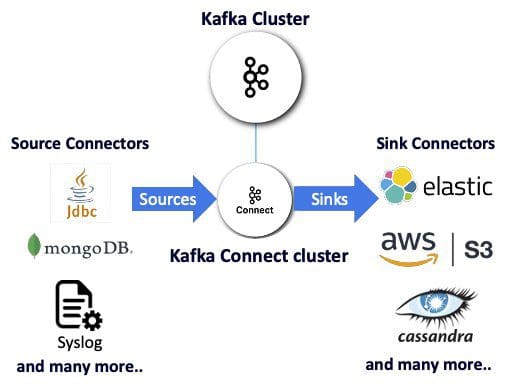
Kafka Connect is a particularly powerful open source data streaming tool that makes it pretty darn painless to pair Kafka with other data technologies. As a distributed technology, Kafka Connect offers particularly high availability and elastic scaling independent of Kafka clusters. Using source or sink connectors to send data to and from Kafka topics, Kafka Connect enables integrations with multiple non-Kafka technologies with no code needed.
Robust open source Kafka connectors are available for many popular data technologies, as is the opportunity to write your own. This article walks through a real-world, real-data use case for how to use Kafka Connect to integrate real-time streaming data from Kafka with Elasticsearch (to enable the scalable search of indexed Kafka records) and Kibana (in order to visualize those results).

For an interesting use case that highlights the advantages of Kafka and Kafka Connect, I was inspired by the CDC’s COVID-19 data tracker. The Kafka-enabled tracker collects real-time COVID testing data from multiple locations, in multiple formats and using multiple protocols, and processes those events into easily-consumable, visualized results. The tracker also has the necessary data governance to make sure results arrive quickly and can be trusted.
I began searching for a similarly complex and compelling use case – but ideally one less fraught than the pandemic. Eventually I came upon an interesting domain, one that included publicly available streaming REST APIs and rich data in a simple JSON format: lunar tides.
Lunar tide data
Tides follow the lunar day, a 24-hour-50-minute period during which the planet fully rotates to the same point beneath the orbiting moon. Each lunar day has two high tides and two low tides caused by the moon’s gravitational pull:

Source 1 National Oceanic and Atmospheric Administration
The National Oceanic and Atmospheric Administration (NOAA) provides a REST API that makes it easy to retrieve detailed sensor data from its global tidal stations.

For example, the following REST call specifies the station ID, data type (I chose sea level) and datum (mean sea level), and requests the single more recent result in metric units:
https://api.tidesandcurrents.noaa.gov/api/prod/datagetter?date=latest&station=8724580&product=water_level&datum=msl&units=metric&time_zone=gmt&application=instaclustr&format=json
This call returns a JSON result with the latitude and longitude of the station, the time, and the water level value. Note that you must remember what your call was in order to understand the data type, datum, and units of the returned results!
{"metadata": {
   "id":"8724580",
   "name":"Key West",
   "lat":"24.5508”,
   "lon":"-81.8081"},
 "data":[{
   "t":"2020-09-24 04:18",
   "v":"0.597",
      "s":"0.005", "f":"1,0,0,0", "q":"p"}]}
Starting the data pipeline (with a REST source connector)
To begin creating the Kafka Connect streaming data pipeline, we must first prepare a Kafka cluster and a Kafka Connect cluster.

Next, we introduce a REST connector, such as this available open source one. We’ll deploy it to an AWS S3 bucket (use these instructions if needed). Then we’ll tell the Kafka Connect cluster to use the S3 bucket, sync it to be visible within the cluster, configure the connector, and finally get it running. This “BYOC” (Bring Your Own Connector) approach ensures that you have limitless options for finding a connector that meets your specific needs.

The following example demonstrates using a “curl” command to configure a 100% open source Kafka Connect deployment to use a REST API. Note that you’ll need to change the URL, name, and password to match your own deployment:
curl https://connectorClusterIP:8083/connectors -k -u name:password -X POST -H 'Content-Type: application/json' -d '

{
    "name": "source_rest_tide_1",
    "config": {
      "key.converter":"org.apache.kafka.connect.storage.StringConverter",
      "value.converter":"org.apache.kafka.connect.storage.StringConverter",
      "connector.class": "com.tm.kafka.connect.rest.RestSourceConnector",
      "tasks.max": "1",
      "rest.source.poll.interval.ms": "600000",
      "rest.source.method": "GET",
      "rest.source.url": "https://api.tidesandcurrents.noaa.gov/api/prod/datagetter?date=latest&station=8454000&product=water_level&datum=msl&units=metric&time_zone=gmt&application=instaclustr&format=json",
      "rest.source.headers": "Content-Type:application/json,Accept:application/json",
      "rest.source.topic.selector": "com.tm.kafka.connect.rest.selector.SimpleTopicSelector",
      "rest.source.destination.topics": "tides-topic"
    }
}
The connector task created by this code polls the REST API in 10-minute intervals, writing the result to the “tides-topic” Kafka topic. By randomly choosing five total tidal sensors to collect data this way, tidal data is now filling the tides topic via five configurations and five connectors.

Ending the pipeline (with an Elasticsearch sink connector)
To give this tide data somewhere to go, we’ll introduce an Elasticsearch cluster and Kibana at the end of the pipeline. We’ll configure an open source Elasticsearch sink connector to send Elasticsearch the data.

The following sample configuration uses the sink name, class, Elasticsearch index, and our Kafka topic. If an index doesn’t exist already, one with default mappings will be created.
curl https://connectorClusterIP:8083/connectors -k -u name:password -X POST -H 'Content-Type: application/json' -d '
{
  "name" : "elastic-sink-tides",
  "config" :
  {
    "connector.class" : "com.datamountaineer.streamreactor.connect.elastic7.ElasticSinkConnector",
    "tasks.max" : 3,
    "topics" : "tides",
    "connect.elastic.hosts" : ”ip",
    "connect.elastic.port" : 9201,
    "connect.elastic.kcql" : "INSERT INTO tides-index SELECT * FROM tides-topic",
    "connect.elastic.use.http.username" : ”elasticName",
    "connect.elastic.use.http.password" : ”elasticPassword"
  }
}'
The pipeline is now operational. However, all tide data arriving in the Tides index is a string, due to the default index mappings.

Custom mapping is required to correctly graph our time series data. We’ll create this custom mapping for the tides-index below, using the JSON “t” field for the custom date, “v” as a double, and “name” as the keyword for aggregation:
curl -u elasticName:elasticPassword ”elasticURL:9201/tides-index"  -X PUT -H 'Content-Type: application/json' -d'
{
"mappings" : {
  "properties" : {
     "data" : {
        "properties" : {
             "t" : { "type" : "date",
                     "format" : "yyyy-MM-dd HH:mm"
             },
             "v" : { "type" : "double" },
             "f" : { "type" : "text" },
             "q" : { "type" : "text" },
             "s" : { "type" : "text" }
             }
       },
       "metadata" : {
          "properties" : {
             "id" : { "type" : "text" },
             "lat" : { "type" : "text" },
             "long" : { "type" : "text" },
             "name" : { "type" : ”keyword" } }}}}         }'
Elasticsearch “reindexing” (deleting the index and reindexing all data) is typically required each time you change an Elasticsearch index mapping. Data can either be replayed from an existing Kafka sink connector, as we have in this use case, or sourced using the Elasticsearch reindex operation.
Visualizing data with Kibana
To visualize the tide data, we’ll first create an index pattern in Kibana, with “t” configured as the timefilter field. We’ll then create a visualization, choosing a line graph type. Lastly, we’ll configure the graph settings such that the y-axis displays the average tide level over 30 minutes and the x-axis shows that data over time.
The result is a graph of changes in the tides for the five sample stations that the pipeline collects data from:

Results
The periodic nature of tides is plain to see in our visualization, with two high tides occurring each lunar day.

More surprisingly, the range between high and low tides is different at each global station. This is due to the influences of not just the moon, but the sun, local geography, weather, and climate change. This example Kafka Connect pipeline utilizes Kafka, Elasticsearch and Kibana to helpfully demonstrate the power of visualizations: they can often reveal what raw data cannot!
Bio: Paul Brebner is the Technology Evangelist at Instaclustr, which provides a managed service platform of open source technologies such as Apache Cassandra, Apache Spark, OpenSearch, Redis, and Apache Kafka.
Related:
- 5 Python Data Processing Tips & Code Snippets
- What’s ETL?
- Date Processing and Feature Engineering in Python