Generate Synthetic Time-series Data with Open-source Tools
An introduction to the generative adversarial network model DoppelGANger, and how you can use a new open-source PyTorch implementation of it to create high-quality synthetic time-series data.

Introduction
Time series data, a sequence of measurements of the same variables across multiple points in time, is ubiquitous in the modern data world. Just as with tabular data, we often want to generate synthetic time series data to protect sensitive information or create more training data when real data is rare. Some applications for synthetic time series data include sensor readings, timestamped log messages, financial market prices, and medical records. The additional dimension of time where trends and correlations across time are just as important as correlations between variables creates added challenges for synthetic data.
At Gretel, we’ve previously published blogs on synthesizing time series data (financial data, time series basics), but are always looking at new models that can improve our synthetic data generation. We really liked the DoppelGANger model and associated paper (Using GANs for Sharing Networked Time Series Data: Challenges, Initial Promise, and Open Questions by Lin et. al.) and are in the process of incorporating this model into our APIs and console. As part of that work, we reimplemented the DoppelGANger model in PyTorch and are thrilled to release it as part of our open source gretel-synthetics library.
In this article, we give a brief overview of the DoppelGANger model, provide sample usage of our PyTorch implementation, and demonstrate excellent synthetic data quality on a task synthesizing daily wikipedia web traffic with a ~40x runtime speedup compared to the TensorFlow 1 implementation.
DoppelGANger Model
DoppelGANger is based on a generative adversarial network (GAN) with some modifications to better fit the time series generation task. As a GAN, the model uses an adversarial training scheme to simultaneously optimize the discriminator (or critic) and generator networks by comparing synthetic and real data. Once trained, arbitrary amounts of synthetic time-series data can be created by passing input noise to the generator network.
In their paper, Lin et al. review existing synthetic time series approaches and their own observations to identify limitations and propose several specific improvements that make up DoppelGANger. These range from generic GAN improvements, to time-series specific tricks. A few of these key modifications are listed below:
- Generator contains an LSTM to produce sequence data, but with a batch setup where each LSTM cell outputs multiple time points to improve temporal correlations.
- Supports variable-length sequences in both training and generation (planned, but not yet implemented in our PyTorch version). For example, one model can use and create 10 or 15 seconds of sensor measurements.
- Supports fixed variables (attributes) that do not vary over time. This information is often found with time series data, for example, an industry or sector associated with each stock in financial price history data.
- Supports per-example scaling of continuous variables to handle data with large dynamic range. For example, differences of several orders of magnitude in page views for popular versus rare wikipedia pages.
- Uses Wasserstein loss with gradient penalty to reduce mode collapse and improve training.
A small note on terminology and data setup. DoppelGANger requires training data with multiple examples of time series. Each example consists of 0 or more attribute values, fixed variables that do not vary over time, and 1 or more features that are observed at each time point. When combined into a training data set, the examples look like a 2d array of attributes (example x fixed variable) and a 3d array of features (example x time x time variable). Depending on the task and available data, this setup may require splitting a few long time sequences into shorter chunks that can be used as the examples for training.
Overall these modifications to a basic GAN provide an expressive time series model that produces high-fidelity synthetic data. We are particularly impressed with DoppelGANger’s ability to learn and generate data with temporal correlations at different scales, such as weekly and yearly trends. For full details on the model, please read the excellent paper by Lin et. al.
Sample Usage
Our PyTorch implementation supports 2 styles of input (numpy arrays or pandas DataFrame) plus a number of configuration options for the model. For full reference documentation, see https://synthetics.docs.gretel.ai/
The simplest way to use our model is with your training data in a pandas DataFrame. For this setup, the data must be in a “wide” format where each row is an example, some columns may be attributes, and the remaining columns are the time series values. The following snippet demonstrates training and generating data from a DataFrame.
# Create some random training data

df = pd.DataFrame(np.random.random(size=(1000,30)))

df.columns = pd.date_range("2022-01-01", periods=30)

# Include an attribute column

df["attribute"] = np.random.randint(0, 3, size=1000)
# Train the model

model = DGAN(DGANConfig(

   max_sequence_len=30,

   sample_len=3,

   batch_size=1000,

   epochs=10,  # For real data sets, 100-1000 epochs is typical

))
model.train_dataframe(

   df,

   df_attribute_columns=["attribute"],

   attribute_types=[OutputType.DISCRETE],

)
# Generate synthetic data

synthetic_df = model.generate_dataframe(100)
If your data isn’t already in this “wide” format, you may be able to use the pandas pivot method to convert it to the expected structure. The DataFrame input is somewhat limited currently, though we have plans to support other ways of accepting of time series data in the future. For the most control and flexibility, you can also pass numpy arrays directly for training (and similarly receive the attribute and feature arrays back when generating data), demonstrated below.
# Create some random training data

attributes = np.random.randint(0, 3, size=(1000,3))

features = np.random.random(size=(1000,20,2))
# Train the model

model = DGAN(DGANConfig(

   max_sequence_len=20,

   sample_len=4,

   batch_size=1000,

   epochs=10,  # For real data sets, 100-1000 epochs is typical

))
model.train_numpy(

   attributes, features,

   attribute_types = [OutputType.DISCRETE] * 3,

   feature_types = [OutputType.CONTINUOUS] * 2

)
# Generate synthetic data

synthetic_attributes, synthetic_features = model.generate_numpy(1000)
Runnable versions of these snippets are available at sample_usage.ipynb.
Results
As a new implementation that switches from TensorFlow 1 to PyTorch (with potential differences in underlying components such as optimizers, parameter initialization, etc.), we want to confirm our PyTorch code works as expected. To do this, we’ve replicated a selection of results from the original paper. Since our current implementation only supports fixed-length sequences, we focus on a data set of wikipedia web traffic (WWT).
The WWT data set, used by Lin et. al. and originally from Kaggle, contains daily traffic measurements to various wikipedia pages. There are 3 discrete attributes (domain, access type, and agent) associated with each page and a single time series feature of daily page views for 1.5 years (550 days). See Image 1 for a few example time series from the WWT data set.
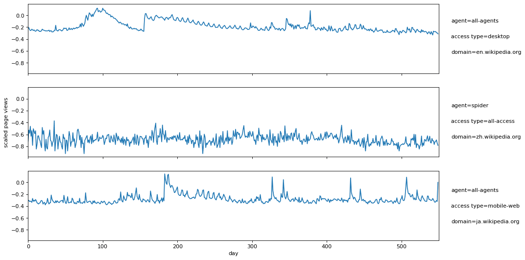
Image 1: Scaled daily page views for 3 wikipedia pages with page attributes listed on the right.
Note the page views are log scaled to [-1,1] based on min/max page views across the entire data set. The training data of 50k pages we used in our experiments (already scaled) is available as a csv on S3.
We present 3 images showing different aspects of the fidelity of the synthetic data. In each image, we compare the real data with 3 synthetic versions: 1) fast PyTorch implementation with larger batch size and smaller learning rate, 2) PyTorch implementation with original parameters, 3) TensorFlow 1 implementation. In Image 2, we look at the distribution of attributes where the synthetic data is a close match to the real distributions (modeled after Figure 19 from the appendix of Lin et. al.).
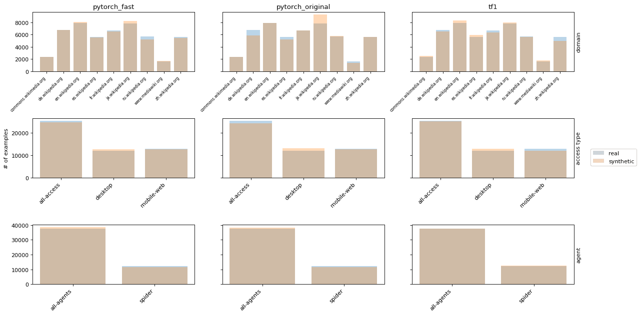
Image 2: Attribute distributions of real and synthetic WWT data.
One of the challenges with the WWT data is that different time series have very different ranges of page views. Some wikipedia pages consistently receive lots of traffic, while others are much less popular, but occasionally get a spike due to some relevant current event, for example, a breaking news story related to the page. Lin et. al. found that DoppelGANger is highly effective at generating time series on different scales (Figure 6 of the original paper). In Image 3, we provide similar plots showing the distribution of time series midpoints. For each example, the midpoint is halfway between the minimum and maximum page views attained over the 550 days. Our PyTorch implementation shows similar fidelity for the midpoints.
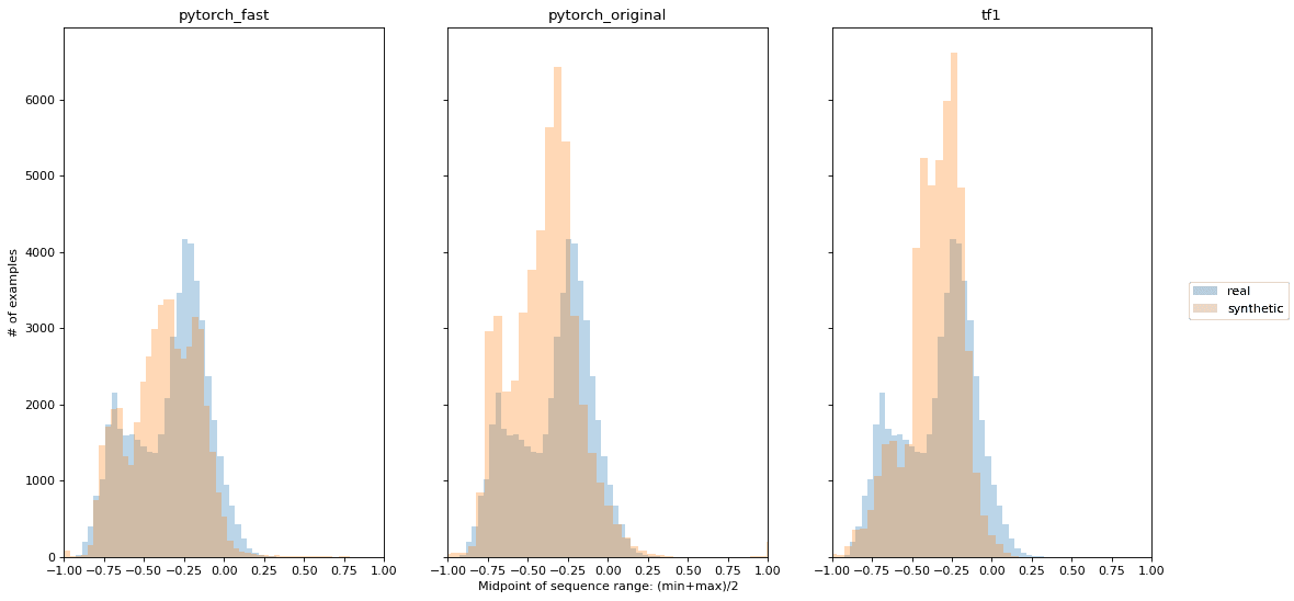
Image 3: Time series midpoint distributions of real and synthetic WWT data.
Lastly, traffic to most wikipedia pages exhibits weekly and yearly patterns. To evaluate these patterns, we use autocorrelation, that is, Pearson correlation of page views at different time lags (1 day, 2 days, etc.). Autocorrelation plots for the 3 synthetic versions are shown in Image 4 (similar to Figure 1 of the original paper).
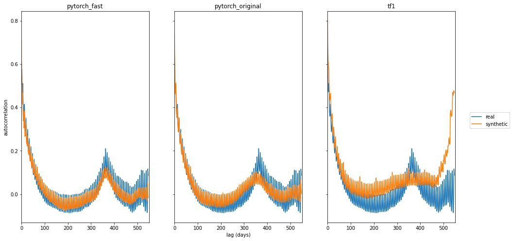
Image 4: Autocorrelation for real and synthetic WWT data.
Both PyTorch versions produce the weekly and yearly trend as observed in the original paper. The TensorFlow 1 results don’t match Figure 1 of Lin et al. exactly as the above plots are from our experiments. We observed somewhat inconsistent training using the original parameters where the model occasionally does not pick up the yearly (or even weekly) pattern. The lower learning rate (1e-4) and larger batch size (1000) used in our fast version makes retrainings more consistent.
Analysis code to produce the images in this section and to train the 3 models are shared as notebooks on github.
Runtime
Last but not least, a crucial aspect of more complex models is runtime. An amazing model that takes weeks to train is much more practically limited than one that takes an hour to train. Here, the PyTorch implementation compares extremely well (though as the authors note in their paper, they did not do performance optimization on the TensorFlow 1 code). All models were trained using the GPU and ran on GCP n1-standard-8 instances (8 virtual CPUs, 30 GB RAM) with an NVIDIA Tesla T4. Going from 13 hours to 0.3 hours is crucial for making this impressive model more useful in practice!
| Version | Training time |
| TensorFlow 1 | 12.9 hours |
| PyTorch, batch_size=100 (original parameters) | 1.6 hours |
| PyTorch, batch_size=1000 | 0.3 hours |
Conclusion
Gretel.ai has added a PyTorch implementation of the DoppelGANger time series model to our open-source gretel-synthetics library. We showed this implementation produces high-quality synthetic data, and is substantially faster (~40x) than the previous TensorFlow 1 implementation. If you enjoyed this post, leave a ⭐ on our gretel-synthetics GitHub, and let us know on our Slack if you have any questions! Please watch for more blogs on time series as we incorporate DoppelGANger into our APIs and add additional features such as support for variable-length sequences.
Credits
Thanks to the authors of the excellent DoppelGANger paper: Using GANs for Sharing Networked Time Series Data: Challenges, Initial Promise, and Open Questions by Zinan Lin, Alankar Jain, Chen Wang, Giulia Fanti, Vyas Sekar. And we’re especially grateful to Zinan Lin for responding to questions about the paper and TensorFlow 1 code.
Kendrick Boyd is Principal ML Engineer at Gretel.ai.