Dimensionality Reduction Techniques in Data Science
Dimensionality reduction techniques are basically a part of the data pre-processing step, performed before training the model.
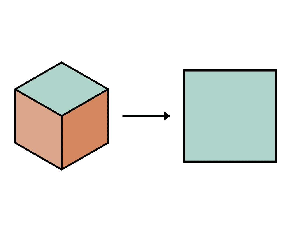
Image by Editor
Introduction
Analyzing data with a list of variables in machine learning requires a lot of resources and computations, not to mention the manual labor that goes with it. This is precisely where the dimensionality reduction techniques come into the picture. The dimensionality reduction technique is a process that transforms a high-dimensional dataset into a lower-dimensional dataset without losing the valuable properties of the original data. These dimensionality reduction techniques are basically a part of the data pre-processing step, performed before training the model.
What is Dimensionality Reduction in Data Science?
Imagine you are training a model that could predict the next day's weather based on the various climatic conditions of the present day. The present-day conditions could be based on sunlight, humidity, cold, temperature, and many millions of such environmental features, which are too complex to analyze. Hence, we can lessen the number of features by observing which of them are strongly correlated with each other and clubbing them into one.
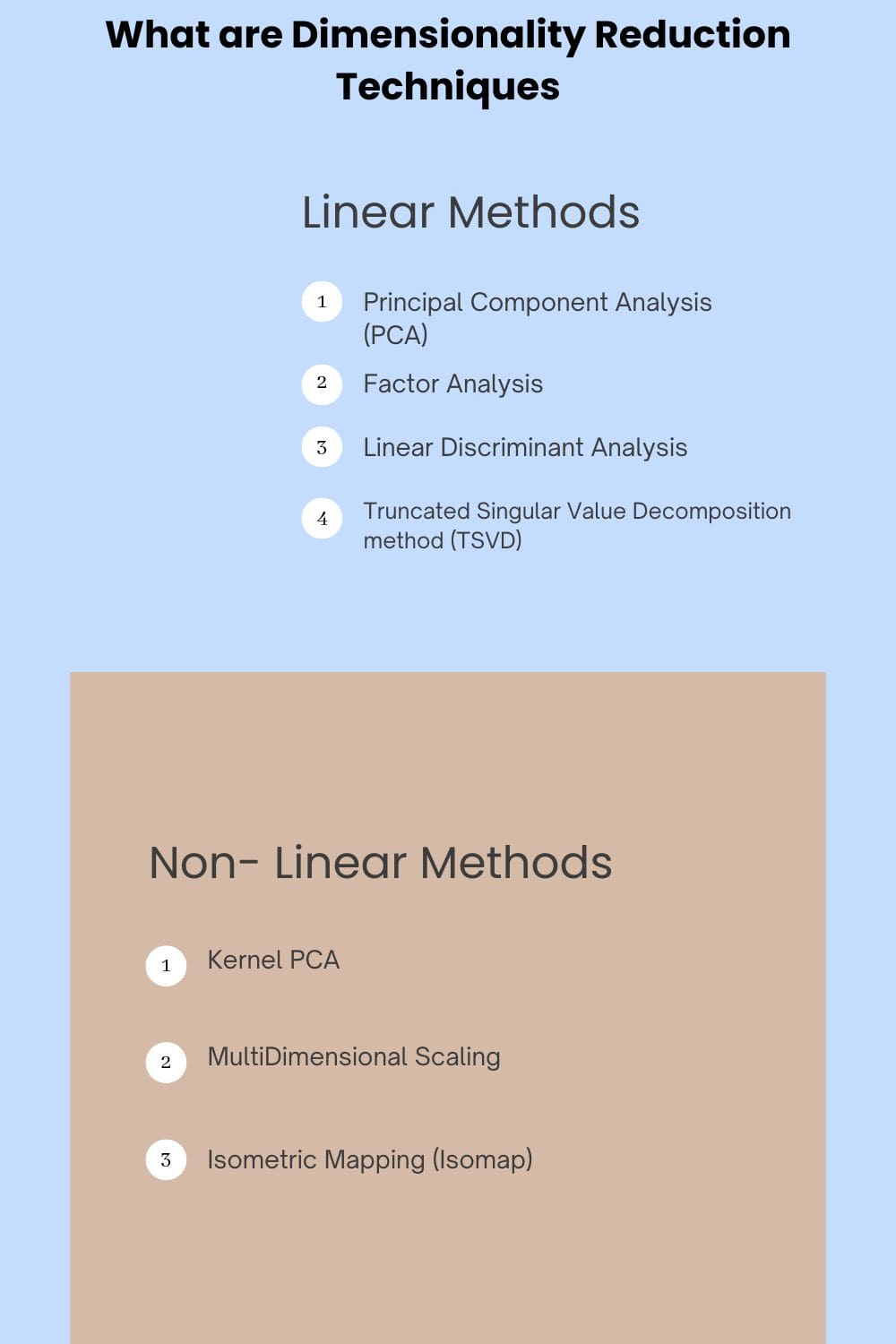
image by Auhtor
Here, we can club humidity and rainfall into a single dependent feature since we know they are strongly correlated. That's it! This is how the dimensionality reduction technique is used to compress complex data into a simpler form without losing the essence of the data. Moreover, data science and AI experts are now also using data science solutions to leverage business ROI. Data visualization, data mining, predictive analytics, and other data analytics services by Datatobiz are changing the business game.
Why is Dimensionality Reduction Necessary?
machine learning and Deep Learning techniques are performed by inputting a vast amount of data to learn about fluctuations, trends, and patterns. Unfortunately, such huge data consists of many features, which often leads to a curse of dimensionality.
Moreover, sparsity is a common occurrence in large datasets. Sparsity refers to having negligible or no value features, and if it is inputted in a training model, it performs poorly on testing. In addition, such redundant features cause problems in clustering the similar features of the data.
Hence, to counter the curse of dimensionality, dimensionality reduction techniques come to the rescue. The answers to the question of why dimensionality reduction is useful are:
- The model performs more accurately since redundant data will be removed, which will lead to less room for assumption.
- Less usage of computational resources, which will save time and financial budget
- A few machine learning/Deep Learning techniques do not work on high-dimensional data, a problem that will be solved once the dimension reduces.
- Clean and non-sparse data will give rise to more statistically significant results because clustering of such data is easier and more accurate.
Now let us understand which algorithms are used for dimensionality reduction of data with examples.
What are Dimensionality Reduction Techniques
The dimensionality reduction techniques are broadly divided into two categories, namely,
- Linear Methods
- Non-Linear Methods
1. Linear Methods
PCA
Principal Component Analysis (PCA) is one of the used DR techniques in data science. Consider a set of 'p' variables that are correlated with each other. This technique reduces this set of 'p' variables into a smaller number of uncorrelated variables, usually denoted by 'k', where (k<p). These 'k' variables are called principal components, and their variation is similar to the original dataset.
PCA is used to figure out the correlation among features, which it combines together. As a result, the resultant dataset has lesser features that are linearly correlated with each other. This way, the model performs the reduction of correlated features while simultaneously calculating maximum variance in the original dataset. After finding the directions of this variance, it directs them into a smaller dimensional space which gives rise to new components called principal components.
These components are pretty sufficient in representing the original features. Therefore, it reduces the reconstruction error while finding out the optimum components. This way, data is reduced, making the machine learning algorithms perform better and faster. PrepAI is one of the perfect examples of AI that has made use of the PCA technique in the backend to generate questions from a given raw text intelligently.
Factor Analysis
This technique is an extension of Principal Component Analysis (PCA). The main focus of this technique is not just to reduce the dataset. It focuses more on finding out latent variables, which are results of other variables from the dataset. They are not measured directly in a single variable.
Latent variables are also called factors. Hence, the process of building a model which measures these latent variables is known as factor analysis. It not only helps in reducing the variables but also helps in distinguishing response clusters. For example, you have to build a model which will predict customer satisfaction. You will prepare a questionnaire that has questions like,
"Are you happy with our product?"
"Would you share your experience with your acquaintances?"
If you want to create a variable to rate customer satisfaction, you will either average the responses or create a factor-dependent variable. This can be performed using PCA and keeping the first factor as a principal component.
Linear Discriminant Analysis
It is a dimensionality reduction technique that is used mainly for supervised classification problems. Logistic Regression fails in multi-classification. Hence, LDA comes into the picture to counter that shortcoming. It efficiently discriminates between training variables in their respective classes. Moreover, it is different from PCA as it calculates a linear combination between the input features to optimize the process of distinguishing different classes.
Here is an example to help you understand LDA:
Consider a set of balls belonging to two classes: Red Balls and Blue Balls. Imagine they are plotted on a 2D plane randomly, such that they cannot be separated into two distinct classes using a straight line. In such cases, LDA is used, which can convert a 2D graph into a 1D graph, thereby maximizing the distinction between the classes of balls. The balls are projected to a new axis which separates them into their classes in the best possible way. The new axis is formed using two steps:
- By maximizing the distances between the means of two classes
- By minimizing the variation within each individual class
SVD
Consider data with 'm' columns. Truncated Singular Value Decomposition method (TSVD) is a projection method where these 'm' columns (features) are projected into a subspace with 'm' or lesser columns without losing the characteristics of the data.
An example where TSVD can be used is a dataset containing reviews about e-commerce products. The review column is mostly left blank, which gives rise to null values in the data, and TSVD tackles it efficiently. This method can be implemented easily using the TruncatedSVD() function.
While the PCA uses dense data, SVD uses sparse data. Moreover, the covariance matrix is used for PCA factorization, whereas TSVD is done on a data matrix.
2. Non-Linear Methods
Kernel PCA
PCA is quite efficient for datasets that are linearly separable. However, if we apply it to datasets that are non-linear, the reduced dimension of the dataset may not be accurate. Hence, this is where Kernel PCA becomes efficient.
The dataset undergoes a kernel function and is temporarily projected into a higher dimensional feature space. Here, the classes are transformed and can be separated linearly and distinguished with the help of a straight line. Further, a general PCA is applied, and the data is projected back onto a reduced dimensional space. Conducting this linear dimensionality reduction method in that space will be as good as conducting non-linear dimensionality reduction in the actual space.
Kernel PCA operates on 3 important hyperparameters: the number of components we wish to retain, the type of kernel we want to use, and the kernel coefficient. There are different types of the kernel, namely, 'linear', 'poly', 'rbf', 'sigmoid', 'cosine'. Radial Basis Function kernel (RBF) is widely used among them.
T-Distributed Stochastic Neighbor Embedding
It is a non-linear dimensionality reduction method primarily applied for data visualization, image processing, and NLP. T-SNE has a flexible parameter, namely, 'perplexity'. It showcases how to maintain attendance between global and local aspects of the dataset. It gives an estimate of the number of close neighbors of each data point. Also, it transforms the similarities between different data points into joint probabilities, and the Kullback-Leibler divergence is minimized between the joint probabilities of low-dimensional embedding and high-dimensional datasets. Moreover, T-SNE also comes up with a cost function that is not convex in nature, and with different initializations, one can get different results.
T-SNE preserves only minimum pairwise distances or local similarities, while PCA preserves maximum pairwise distances to maximize variance. Also, PCA or TSVD is highly recommended to reduce the dimensions of the features in the dataset to exceed more than 50 because T-SNE fails in this case.
Multi-Dimensional Scaling
Scaling refers to making the data simpler by reducing it to a lower dimension. It is a non-linear dimensionality reduction technique that showcases the distances or dissimilarities between the sets of features in a visualized manner. Features with shorter distances are considered similar, whereas those with larger distances are dissimilar.
MDS reduces the data dimension and interprets the dissimilarities in the data. Also, data doesn't lose its essence after scaling down; two data points will always be at the same distance irrespective of their dimension. This technique can only be applied to matrices having relational data, such as correlations, distances, etc. Let's understand this with the help of an example.
Consider you have to make a map, where you are provided with a list of city locations. The map should also showcase the distances between the two cities. The only possible method to do this would be to measure the distances between the cities with the help of a meter tape. But what if you are only provided with the distances between the cities and their similarities instead of the city locations? You could still draw a map using logical assumptions and a wide knowledge of geometry.
Here, you are basically applying MDS to create a map. MDS observes the differences in the dataset and creates a map that calculates the original distances and tells you where they are located.
Isometric Mapping (Isomap)
It is a non-linear dimensionality reduction technique that is basically an extension of MDS or Kernel PCA. It reduces dimensionality by connecting every feature on the basis of their curved or geodesic distances between their nearest neighbors.
Isomap is initiated by building a neighborhood network. Then, it uses graph distance to estimate the geodesic distance between every pair of points. Finally, the dataset is embedded in a lower dimension by decomposing the eigenvalues of the geodesic matrix. It can be specified how many neighbors to consider for each data point using the n_neighbours hyperparameter of the Isomap() class. This class implements the Isomap algorithm.
What is the need for Dimensionality Reduction in Data Mining?
Data mining is the process of observing hidden patterns, relations, and anomalies within vast datasets in order to estimate outcomes. Vast datasets have many variables increasing at an exponential rate. Therefore, finding and analyzing patterns in them during the data mining process takes lots of resources and computational time. Hence, the dimensionality reduction technique can be applied while data mining to limit those data features by clubbing them and still be sufficient enough to represent the original dataset.
Advantages and Disadvantages of Dimensionality Reduction
Advantages
- Storage space and the processing time are less
- Multi-collinearity of the dependent variables is removed
- Reduced chances of overfitting the model
- Data Visualization becomes easier
Disadvantages
- Some amount of data is lost.
- PCA cannot be applied where data cannot be defined through mean and covariance.
- Not every variable needs to be linearly correlated, which PCA tends to find.
- Labeled data is required for LDA to function, which is not available in a few cases.
Conclusion
A vast amount of data is generated every second. So, analyzing them with optimal use of resources and with accuracy is equally important. Dimensionality Reduction techniques help in data pre-processing in a precise and efficient manner—no wonder why it is considered a boon for data scientists.
Kavika Roy is Head of Information Management at DataToBiz. She is responsible for the identification, acquisition, distribution, and organization of technical oversight. Her strong attention to detail lets her deliver precise information regarding functional aspects to the right audience.