PySpark for Data Science
In this tutorial, we will learn to Initiates the Spark session, load, and process the data, perform data analysis, and train a machine learning model.
Image by Author
PySpark is an Python interference for Apache Spark. It is an open-source library that allows you to build Spark applications and analyze the data in a distributed environment using a PySpark shell. You can use PySpark for batch processing, running SQL queries, Dataframes, real-time analytics, machine learning, and graph processing.
Advantages of using Spark:
- In-memory caching allows real-time computation and low latency.
- It can be deployed using multiple ways: Spark’s cluster manager, Mesos, and Hadoop via Yarn.
- User-friendly API is available for all popular languages that hide the complexity of running distributed systems.
- It is 100x faster than Hadoop MapReduce in memory and 10x faster on disk.
In this code-based tutorial, we will learn how to initial spark session, load the data, change the schema, run SQL queries, visualize the data, and train the machine learning model.
Getting Started
If you want to use PySpark on a local machine, you need to install Python, Java, Apache Spark, and PySpark. If you want to avoid all of that, you can use Google Colab or Kaggle. Both platforms come with pre-installed libraries, and you can start coding within seconds.
In the Google Colab Notebook, we will start by installing pyspark and py4j.
%pip install pyspark py4j -qq
After that, we will need to provide the session name to initialize the Spark session.
from pyspark.sql import SparkSession

spark = SparkSession.builder.appName('PySpark_for_DataScience').getOrCreate()
Importing the Data using PySpark
In this tutorial, we will be using Global Spotify Weekly Chart from Kaggle. It contains information about the artist and the songs on the Spotify global weekly chart.
Just like Pandas, we can load the data from CSV to dataframe using spark.read.csv function and display Schema using printSchema() function.
df = spark.read.csv(
    '/content/spotify_weekly_chart.csv',
    sep = ',',
    header = True,
    )

df.printSchema()
Output:
As we can observe, PySpark has loaded all of the columns as a string. To perform exploratory data analysis, we need to change the Schema.
root
 |-- Pos: string (nullable = true)
 |-- P+: string (nullable = true)
 |-- Artist: string (nullable = true)
 |-- Title: string (nullable = true)
 |-- Wks: string (nullable = true)
 |-- Pk: string (nullable = true)
 |-- (x?): string (nullable = true)
 |-- Streams: string (nullable = true)
 |-- Streams+: string (nullable = true)
 |-- Total: string (nullable = true)
Updating the Schema
To change the schema, we need to create a new data schema that we will add to StructType function. You need to make sure that each column field is getting the right data type.
from pyspark.sql.types import *

data_schema = [
               StructField('Pos', IntegerType(), True),
               StructField('P+', StringType(), True),
               StructField('Artist', StringType(), True),
               StructField('Title', StringType(), True),
               StructField('Wks', IntegerType(), True),
               StructField('Pk', IntegerType(), True),
               StructField('(x?)', StringType(), True),
               StructField('Streams', IntegerType(), True),
               StructField('Streams+', DoubleType(), True),
               StructField('Total', IntegerType(), True),
            ]

final_struc = StructType(fields = data_schema)
Then, we will load the CSV files using extra argument schema. After that, we will print the schema to check if the correct changes were made.
df = spark.read.csv(
    '/content/spotify_weekly_chart.csv',
    sep = ',',
    header = True,
    schema = final_struc
    )

df.printSchema()
Output:
As we can see, we have different data types for the columns.
root
 |-- Pos: integer (nullable = true)
 |-- P+: string (nullable = true)
 |-- Artist: string (nullable = true)
 |-- Title: string (nullable = true)
 |-- Wks: integer (nullable = true)
 |-- Pk: integer (nullable = true)
 |-- (x?): string (nullable = true)
 |-- Streams: integer (nullable = true)
 |-- Streams+: double (nullable = true)
 |-- Total: integer (nullable = true)
Exploring the Data
You can explore your data as a dataframe by using toPandas() function.
Note: we have used
limitto display the first five rows. It is similar to SQL commands. This means that we can use PySpark Python API for SQL command to run queries.
df.limit(5).toPandas()
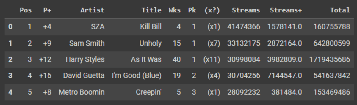
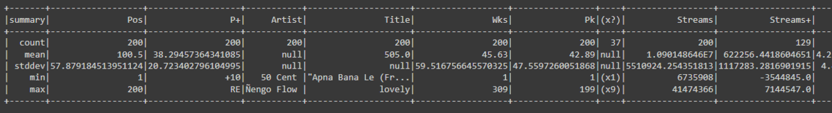
Just like pandas, we can use describe() function to display a summary of data distribution.
df.describe().show()
The count() function used for displaying number of rows. Read Pandas API on Spark to learn about similar APIs.
df.count()
# 200
Column Manipulation
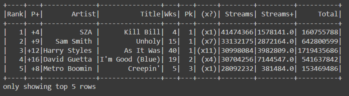
You can rename your column by using withColumnRenamed function. It requires an old name and a new name as string.
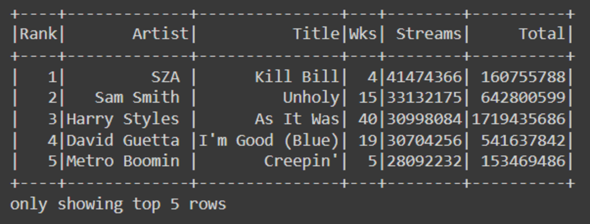
df = df.withColumnRenamed('Pos', 'Rank')

df.show(5)
To drop single or multiple columns, you can use drop() function.
df = df.drop('P+','Pk','(x?)','Streams+')

df.show(5)
You can use .na for dealing with missing valuse. In our case, we are dropping all missing values rows.
df = df.na.drop()
## Or
#data.na.replace(old_value, new_vallue)
Data Analysis
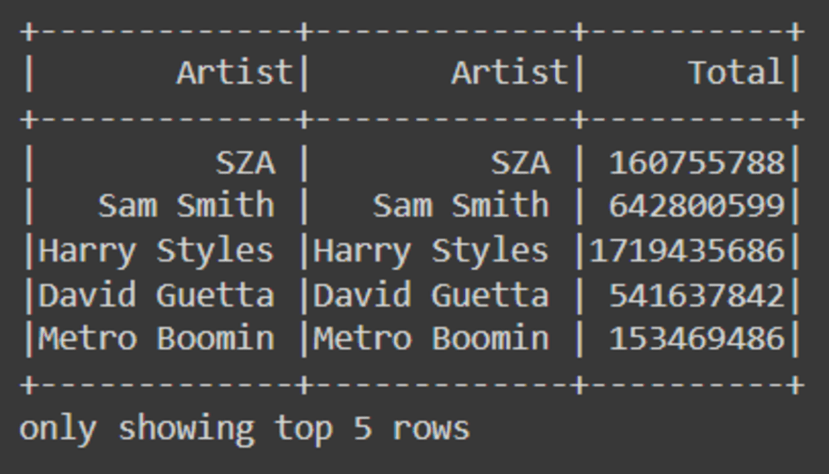
For data analysis, we will be using PySpark API to translate SQL commands. In the first example, we are selecting three columns and display the top 5 rows.
df.select(['Artist', 'Artist', 'Total']).show(5)
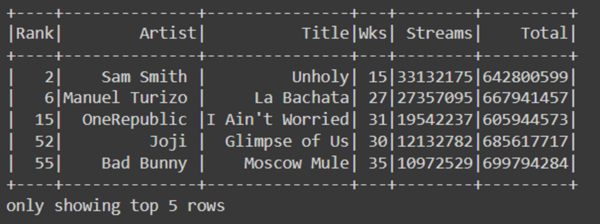
For more complex queries, we will filter values where ‘Total’ is greater than or equal to 600 million to 700 million.
Note: you can also use df.Total.between(600000000, 700000000)to filter out records.
from pyspark.sql.functions import col, lit, when

df.filter(
    (col("Total") >= lit("600000000")) & (col("Total") <= lit("700000000"))
).show(5)
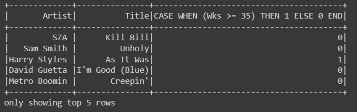
Write if/else statement to create a categorical column using when function.
df.select('Artist', 'Title',
            when(df.Wks >= 35, 1).otherwise(0)
           ).show(5)
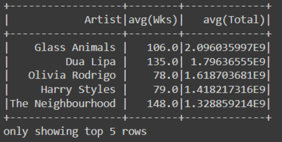
You can use all of the SQL commands as Python API to run a complete query.
df.select(['Artist','Wks','Total'])\
        .groupBy('Artist')\
        .mean()\
        .orderBy(['avg(Total)'], ascending = [False])\
        .show(5)
Data Visualization
Let’s take above query and try to display it as a bar chart. We are plotting “artists v.s average song streams” and we are only displaying the top seven artists.
It is awesome, if you ask me.
vis_df = (
    df.select(["Artist", "Wks", "Total"])
    .groupBy("Artist")
    .mean()
    .orderBy(["avg(Total)"], ascending=[False])
    .toPandas()
)

vis_df.iloc[0:7].plot(
    kind="bar",
    x="Artist",
    y="avg(Total)",
    figsize=(12, 6),
    ylabel="Average Average Streams",
)
Saving the Result
After processing the data and running analysis, it is the time for saving the results.
You can save the results in all of the popular file types, such as CSV, JSON, and Parquet.
final_data = (
    df.select(["Artist", "Wks", "Total"])
    .groupBy("Artist")
    .mean()
    .orderBy(["avg(Total)"], ascending=[False])
)

# CSV
final_data.write.csv("dataset.csv")

# JSON
final_data.write.save("dataset.json", format="json")

# Parquet
final_data.write.save("dataset.parquet", format="parquet")
Data Pre-Processing
In this section, we are preparing the data for the machine learning model.
- Categorical Encoding: converting the categorical columns into integers using StringIndexer.
- Assembling Features: assembling important features into one vector column.
- Scaling: scaling the data using the StandardScaler scaling function.
from pyspark.ml.feature import (
VectorAssembler,
StringIndexer,
OneHotEncoder,
StandardScaler,
)
## Categorical Encoding
indexer = StringIndexer(inputCol="Artist", outputCol="Encode_Artist").fit(
final_data
)
encoded_df = indexer.transform(final_data)
## Assembling Features
assemble = VectorAssembler(
inputCols=["Encode_Artist", "avg(Wks)", "avg(Total)"],
outputCol="features",
)
assembled_data = assemble.transform(encoded_df)
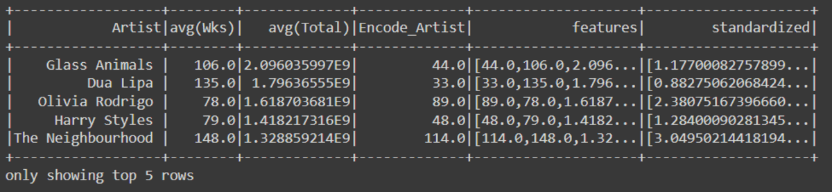
## Standard Scaling
scale = StandardScaler(inputCol="features", outputCol="standardized")
data_scale = scale.fit(assembled_data)
data_scale_output = data_scale.transform(assembled_data)
data_scale_output.show(5)
KMeans Clustering
I have already run the Kmean elbow method to find k. If you want to see all of the code sources with the output, you can check out my notebook.
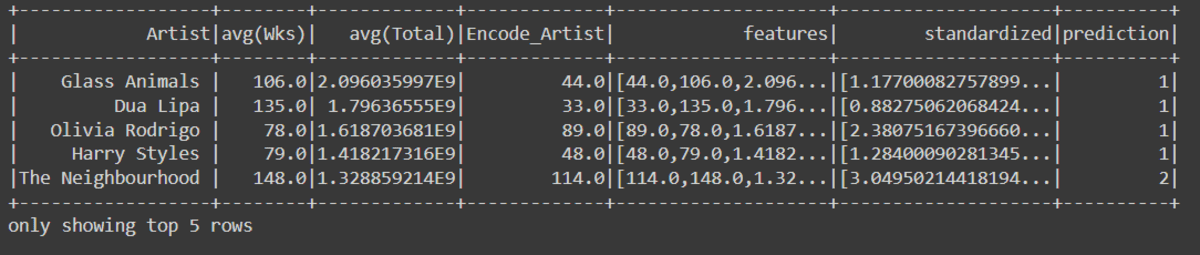
Just like scikit-learn, we will provide a number of clusters and train the Kmeans clustering model.
from pyspark.ml.clustering import KMeans
KMeans_algo=KMeans(featuresCol='standardized', k=4)
KMeans_fit=KMeans_algo.fit(data_scale_output)
preds=KMeans_fit.transform(data_scale_output)

preds.show(5)
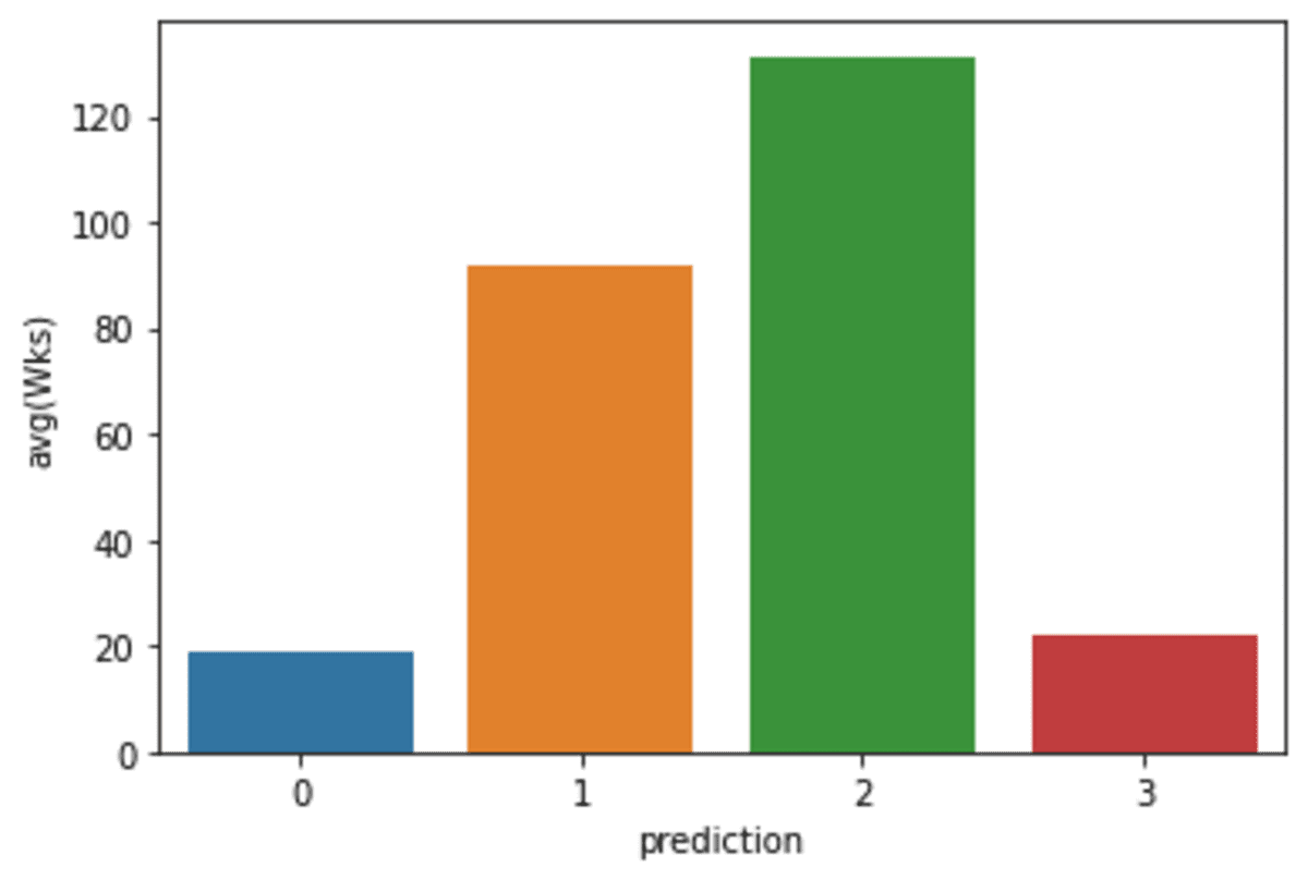
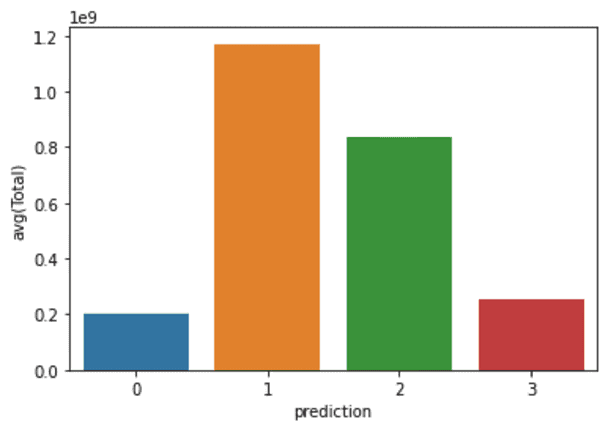
Visualizing Predictions
In this part, we will be using a matplotlib.pyplot.barplot to display the distribution of 4 clusters.
import matplotlib.pyplot as plt
import seaborn as sns

df_viz = preds.select(
    "Artist", "avg(Wks)", "avg(Total)", "prediction"
).toPandas()
avg_df = df_viz.groupby(["prediction"], as_index=False).mean()

list1 = ["avg(Wks)", "avg(Total)"]

for i in list1:
    sns.barplot(x="prediction", y=str(i), data=avg_df)
    plt.show()
Wrapping Up
In this tutorial, I have given an overview of what you can do using PySpark API. The API allows you to perform SQL-like queries, run pandas functions, and training models similar to sci-kit learn. You get the best of all worlds with distributed computing.
It outshines a lot of Python packages when dealing with large datasets (>1GB). If you are a programmer and just interested in Python code, check our Google Colab notebook. You just have to download and add the data from Kaggle to start working on it.
Do let me know in the comments, if you want me to keep writing code based-tutorials for other Python libraries.
Abid Ali Awan (@1abidaliawan) is a certified data scientist professional who loves building machine learning models. Currently, he is focusing on content creation and writing technical blogs on machine learning and data science technologies. Abid holds a Master's degree in Technology Management and a bachelor's degree in Telecommunication Engineering. His vision is to build an AI product using a graph neural network for students struggling with mental illness.