Illustration by Author. Source: Flaticon

Python is the most popular language you’ll encounter in the field of data science for its simplicity, the large community and the huge availability of open-source libraries. 

If you are working on a data science project, Python packages will ease your life since you just need a few lines of code to do complicated operations, like manipulating the data and applying a machine learning/deep learning model.

When starting your data science journey, it’s recommended to start by learning two of the most useful Python packages: NumPy and Pandas. In this article, we are introducing these two libraries. Let’s get started!

What is NumPy?

NumPy stands for Numerical Python and is used to operate efficient computations of arrays and matrices behind the scenes of machine learning models. The building block of Numpy is the array, which is a data structure very similar to the list, with the difference that it provides a huge amount of mathematical functions. In other words, the Numpy array is a multidimensional array object. 

Create Numpy Arrays

We can define NumPy arrays using a list or list of lists:

import numpy as np
l = [[1,2,3],[4,5,6],[7,8,9]]
numpy_array = np.array(l)
numpy_array

array([[1, 2, 3],
       [4, 5, 6],
       [7, 8, 9]])

Differently from a list of lists, we can visualise the matrix 3X3 with an indentation between each row. Moreover, NumPy provides more than 40 built-in functions for array creation. 

To create an array filled with zeros, there is the function np.zeros , in which you just need to specify the shape you desire:

zeros_array = np.zeros((3,4))
zeros_array

array([[0., 0., 0., 0.],
       [0., 0., 0., 0.],
       [0., 0., 0., 0.]])

In the same way, we can create an array filled with ones:

ones_array = np.ones((3,4))
ones_array

array([[1., 1., 1., 1.],
       [1., 1., 1., 1.],
       [1., 1., 1., 1.]])

There is also the possibility to create the identity matrix, which is a square array with 1s on the main diagonal and off-diagonal elements are 0s:

identity_array = np.identity(3)
identity_array

array([[1., 0., 0.],
       [0., 1., 0.],
       [0., 0., 1.]])

Furthermore, NumPy provides different functions to create random arrays. To create an array filled with random samples from a uniform distribution over [0,1], we just need the function np.random.rand :

random_array = np.random.rand(3,4)
random_array

array([[0.84449279, 0.71146992, 0.48159787, 0.04927379],
       [0.03428534, 0.26851667, 0.65718662, 0.52284251],
       [0.1380207 , 0.91146148, 0.74171469, 0.57325424]])

Similarly to the previous function, we can define an array with random values, but this time time are taken from a standard normal distribution:

randn_array = np.random.randn(10)
randn_array

array([-0.68398432, -0.25466784,  0.27020797,  0.29632334, -0.20064897,
        0.7988508 ,  1.34759319, -0.41418478, -0.35223377, -0.10282884])

In case, we are interested on building an array with random integers that belong to the interval [low,high), we just need the function np.random.randint :

randint_array = np.random.randint(1,20,20)
randint_array

array([14,  3,  1,  2, 17, 15,  5, 17, 18,  9,  4, 19, 14, 14,  1, 10, 17,
       19,  4,  6])

Indexing and Slicing

Beyond the built-in functions for array creation, another good point of NumPy is that it’s possible to select elements from the array using a set of square brackets. For example, we can try to take the first row of the matrix:

a1 = np.array([[1,2,3],[4,5,6]])
a1[0]

array([1, 2, 3])

Let’s suppose that we want to select the third element of the first row. In this case, we need to specify two indices, the index of the row and the index of the column:

print(a1[0,2]) #3

An alternative is to use a1[0][2], but it’s considered inefficient because it first creates the array containing the first row and, then, it selects the element from that row.

Moreover, we can take slices from the matrix with the syntax start:stop:step inside the brackets, where the stop index is not included. For example, we want again to select the first row, but we just take the first two elements:

print(a1[0,0:2]) 

[1 2]

If we prefer to select all the rows, but we want to extract the first element of each row:

print(a1[:,0])

[1 4]

In addition to the integer array indexing, there is also the boolean array indexing to select the elements from an array. Let’s suppose that we want only the elements that respect the following condition:

a1>5

array([[False, False, False],
       [False, False,  True]])

If we filter the array based on this condition, the output will show only the True elements:

a1[a1>5]

array([6])

Array Manipulation

When working in data science projects, it often happens to reshape an array to a new shape without changing the data. 

For example, we start with an array of dimension 2X3. If we are not sure of our array’s shape, there is the attribute shape that can helps us:

a1 = np.array([[1,2,3],[4,5,6]])
print(a1)
print('Shape of Array: ',a1.shape)

[[1 2 3]
 [4 5 6]]
Shape of Array:  (2, 3)

To reshape the array to the dimension 3X2, we can simply use the function reshape:

a1 = a1.reshape(3,2)
print(a1)
print('Shape of Array: ',a1.shape)

[[1 2]
 [3 4]
 [5 6]]
Shape of Array:  (3, 2)

Another common situation is to turn a multidimensional array into a single dimensional array. This is possible by specifying -1 as shape:

a1 = a1.reshape(-1)
print(a1)
print('Shape of Array: ',a1.shape)

[1 2 3 4 5 6]
Shape of Array:  (6,)

It can also occur that you need to obtain a transposed array:

a1 = np.array([[1,2,3,4,5,6]])
print('Before shape of Array: ',a1.shape)
a1 = a1.T
print(a1)
print('After shape of Array: ',a1.shape)

Before shape of Array:  (1, 6)
[[1]
 [2]
 [3]
 [4]
 [5]
 [6]]
After shape of Array:  (6, 1)

In the same way, you can apply the same transformation using np.transpose(a1). 

Array Multiplication

If you try to build machine learning algorithms from scratch, you’ll surely need to calculate the matrix product of two arrays. This is possible using the function np.matmul when the array have more than 1 dimension:

a1 = np.array([[1,2,3],[4,5,6]])
a2 = np.array([[1,2],[4,5],[7,8]])
print('Shape of Array a1: ',a1.shape)
print('Shape of Array a2: ',a2.shape)
a3 = np.matmul(a1,a2) 
# a3 = a1 @ a2
print(a3)
print('Shape of Array a3: ',a3.shape)

Shape of Array a1:  (2, 3)
Shape of Array a2:  (3, 2)
[[30 36]
 [66 81]]
Shape of Array a3:  (2, 2)

@ can be a shorter alternative to np.matmul. 

If you multiply a matrix with a scalar, np.dot is the best choice:

a1 = np.array([[1,2,3],[4,5,6]])
a3 = np.dot(a1,2)
# a3 = a1 * 2
print(a3)
print('Shape of Array a3: ',a3.shape)

[[ 2  4  6]
 [ 8 10 12]]
Shape of Array a3:  (2, 3)

In this case, * is a shorter alternative to np.dot. 

Mathematical Functions

NumPy provides a huge variety of mathematical functions, such as the trigonometric functions, rounding functions, exponentials, logarithms and so on. You can find the full list here. We are going to show the most important functions that you can apply to your problems.

The exponential and the natural logarithm are surely the most popular and known transformations:

a1 = np.array([[1,2,3],[4,5,6]])
print(np.exp(a1))

[[  2.71828183   7.3890561   20.08553692]
 [ 54.59815003 148.4131591  403.42879349]]

a1 = np.array([[1,2,3],[4,5,6]])
print(np.log(a1))

[[0.         0.69314718 1.09861229]
 [1.38629436 1.60943791 1.79175947]]

If we want to extract the minimum and the maximum in a single line of code, we just need to call the following functions:

a1 = np.array([[1,2,3],[4,5,6]])
print(np.min(a1),np.max(a1))  # 1 6

We can also calculate the square-root from each element of the array:

a1 = np.array([[1,2,3],[4,5,6]])
print(np.sqrt(a1))

[[1.         1.41421356 1.73205081]
 [2.         2.23606798 2.44948974]]

What is Pandas?

Pandas is built on Numpy and is useful for manipulating the dataset. There are two main data structures: Series and Dataframe. While the Series is a sequence of values, the dataframe is a table with rows and columns. In other words, the series is a column of the dataframe. 

Create Series and Dataframe

To build the Series, we can just pass the list of values to the method:

import pandas as pd
type_house = pd.Series(['Loft','Villa'])
type_house

0     Loft
1    Villa
dtype: object

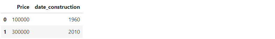
We can create a Dataframe by passing a dictionary of objects, in which the keys correspond to the column names and the values are the entries of the columns:

df = pd.DataFrame({'Price': [100000, 300000], 'date_construction': [1960, 2010]})
df.head()

Once the Dataframe is created, we can check the type of each column:

type(df.Price),type(df.date_construction)

(pandas.core.series.Series, pandas.core.series.Series)

It should be clear that columns are data structures of type Series.

Summary functions

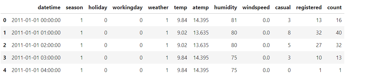
From now on, we show the potentialities of Pandas by using the bike sharing dataset, available on Kaggle. We can import the CSV file in the following way:

df = pd.read_csv('/kaggle/input/bike-sharing-demand/train.csv')
df.head()

Pandas doesn’t only allow reading CSV files, but also Excel file, JSON, Parquet and other types of files. You can find the full list here.

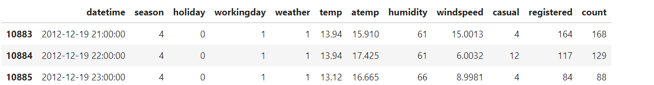
From the output, we can visualise the first five rows of the dataframe. If we want to display the last four rows of the dataset, we use the tail() method:

df.tail(4)

Few rows are not enough to have a good idea of the data we have. A good way of starting the analysis is by looking at the shape of the dataset:

df.shape                    #(10886, 12)

We have 10886 rows and 12 columns. Do you want to see the column names? It’s very intuitive to do:

df.columns

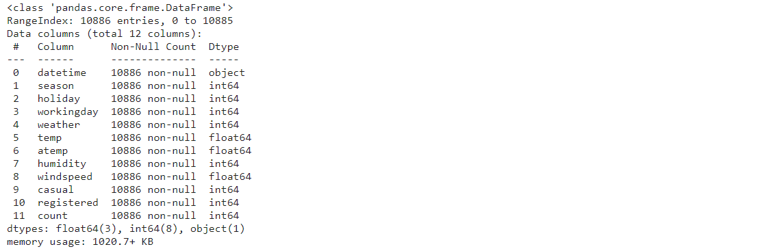
There is a method that allows to visualise all this information into a unique output:

df.info()

If we want to display the statistics of each column, we can use the describe method:

df.describe()

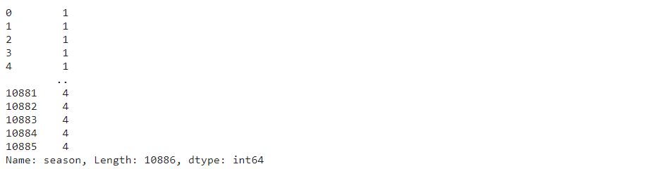
It’s also important to extract information from the categorical fields. We can find the unique values and the number of unique values of the season column:

df.season.unique(),df.season.nunique()

Output:

(array([1, 2, 3, 4]), 4)

We can see that the values are 1, 2, 3,4. Then, there are four possible values. This verification is crucial to understand the categorical variables and prevent possible noise contained in the column.

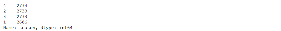
To display the frequency of each level, we can use value_counts() method:

df.season.value_counts()

The last step should be the inspection of the missing values on each column:

df.isnull().sum()

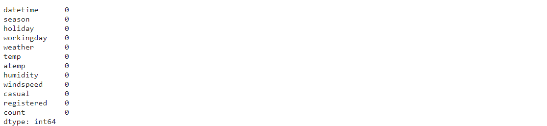
Luckily we don’t have any missing value in any of these fields.

Indexing and Slicing

Like in Numpy, there is the index-based selection to select data from the data structure. There are two main methods to take entries from the dataframe:

• iloc selects the elements based on the integer position
• loc takes the items based on labels or a boolean array.

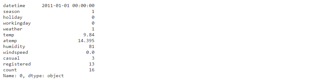
To select the first row, iloc is the best choice:

df.iloc[0]

If we want instead to select all the rows and only the second column, we can do the following:

df.iloc[:,1]

It’s also possible to select more columns at the same time:

df.iloc[0:3,[0,1,2,5]]

It becomes complex to select the columns based on the indices. It would be better to specify the column names. This is possible using loc:

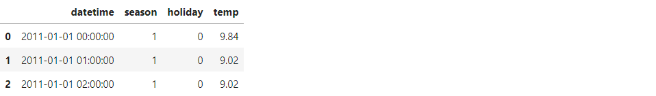
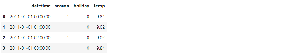
df.loc[0:3,['datetime','season','holiday','temp']]

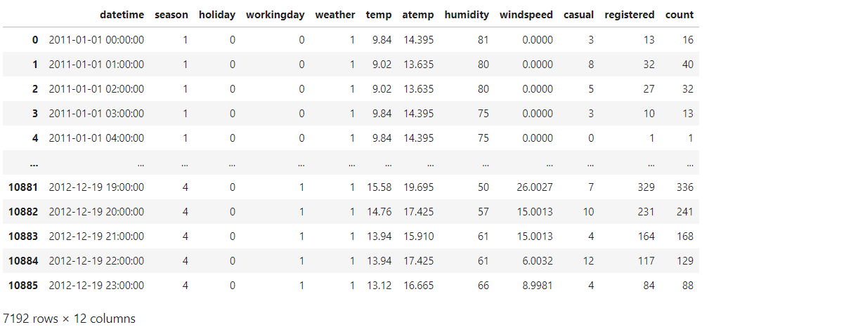
Similarly to Numpy, it’s possible to filter the dataframe based on conditions. For example, we want to return all the rows where weather is equal to 1:

df[df.weather==1]

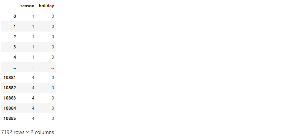
In case we want to return an output with specific columns, we can use loc:

df.loc[df.weather==1,['season','holiday']]

Create new variables

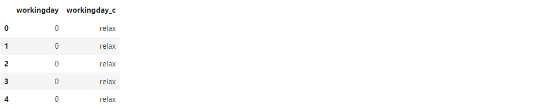
The creation of new variables has a huge impact on extracting more information from the data and improving the interpretability. We can create a new categorical variable based on the values of workingday:

df['workingday_c'] = df['workingday'].apply(lambda x: 'work' if x==1 else 'relax')
df[['workingday','workingday_c']].head()

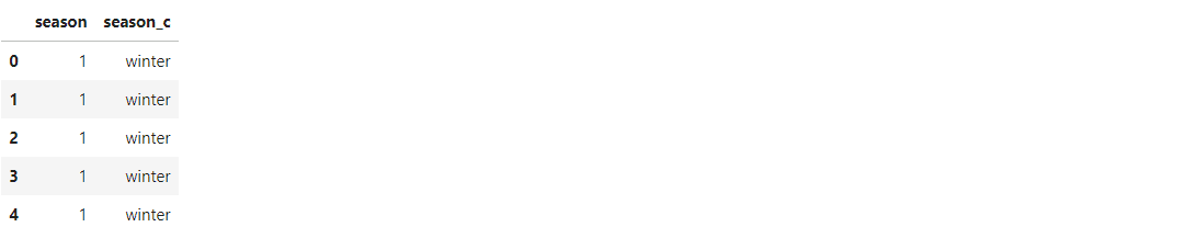
If there are more than one condition, it’s better to map the values using a dictionary and the method map:

diz_season = {1:'winter',2:'spring',3:'summer',4:'fall'}
df['season_c'] = df['season'].map(lambda x: diz_season[x])
df[['season','season_c']].head()

Grouping and Sorting

It can happen that you want to group the data based on categorical column(s). This is possible using groupby:

df.groupby('season_c').agg({'count':['median','max']})

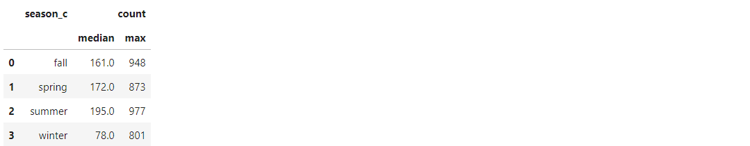
For each level of the season, we can observe the median and the maximum count of rented bikes. This output can be confusing without ordering based on a column. We can do it using the sort_values() method:

df.groupby('season_c').agg({'count':['median','max']}).reset_index().sort_values(by=('count', 'median'),ascending=False)

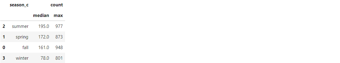
Now, the output makes more sense. We can deduce that the highest number of bikes rented is in summer, while winter is not a good month for renting bikes. 

Final thoughts

That’s it! I hope you have found this guide useful to learn the basics of NumPy and Pandas. They are often studied separately, but it can be insightful to understand first NumPy and then Pandas, which is built on top of NumPy. 

There are surely methods that I didn’t cover within the tutorial, but the goal was to cover the most important and popular methods of these two libraries. The code can be found on Kaggle. Thanks for reading! Have a nice day!
 
 
Eugenia Anello is currently a research fellow at the Department of Information Engineering of the University of Padova, Italy. Her research project is focused on Continual Learning combined with Anomaly Detection.