Linear Regression, Least Squares & Matrix Multiplication: A Concise Technical Overview

Regression is a time-tested manner for approximating relationships among a given collection of data, and the recipient of unhelpful naming via unfortunate circumstances.

Linear regression is a simple algebraic tool which attempts to find the “best” (generally straight) line fitting 2 or more attributes, with one attribute (simple linear regression), or a combination of several (multiple linear regression), being used to predict another, the class attribute. A set of training instances is used to compute the linear model, with one attribute, or a set of attributes, being plotted against another. The model then attempts to identify where new instances would lie on the regression line, given a particular class attribute.

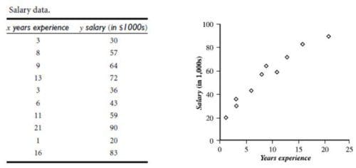
Fig.1: Plotting Data, Preparing for Linear Regression (Han, Kamber & Pei).

The relationship between response and predictor variables (y and x, respectively) can be expressed via the following equation, with which everyone reading this is undoubtedly familiar:

m and b are the regression coefficients, and denote line slope and y-intercept, respectively. I suggest you check your elementary school algebra notes if you are having trouble recalling :)

The equation for multiple linear regression is generalized for n attributes as follows:

It is often confusing for people without a sufficient math background to understand how matrix multiplication fits into linear regression.

Least Squares Method & Matrix Multiplication

One method of approaching linear analysis is the Least Squares Method, which minimizes the sum of the squared residuals. Residuals are the differences between the model fitted value and an observed value, or the predicted and actual values. The exercise of minimizing these residuals would be the trial and error fitting of a line "through" the Cartesian coordinates representing these values.

One way to proceed with the Least Squares Method is to solve via matrix multiplication. How so? The mathematics which underlie the least squares method can be seen here, while a short video with example is shown below.

If you are interested in a video with some additional insight, a proof, and some further examples, have a look here. A number of linear regression for machine learning implementations are available, examples of which include those in the popular Scikit-learn library for Python and the formerly-popular Weka Machine Learning Toolkit.

The least squares method can more formally be described as follows:

Given a dataset of points (x₁, y₁ ), (x₂, y₂ ), ..., (x_n, y_n), we derive the matrices:

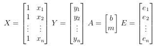
We then set up the matrix equation:

where matrix Y contains the Y values, matrix X contains a row of 1s and along with the X values, matrix A consists of the Y-intercept and slope, and matrix E is the errors. Note the row of 1s in matrix X are needed to allow multiplication with matrix A (2 rows and 2 columns, respectively).

We then solve for A, which is:

This is the matrix equation ultimately used for the least squares method of solving a linear system.

Some Example (Python) Code

The following is a sample implementation of simple linear regression using least squares matrix multiplication, relying on numpy for heavy lifting and matplotlib for visualization.

A particular run of this code generates the following input matrix:

[[ 0.64840322  0.97285346]
 [ 0.77867147  0.87310339]
 [ 0.85072744  0.59023482]
 [ 0.3692784   0.59567815]
 [ 0.14654649  0.79422356]
 [ 0.46897942  0.06988269]
 [ 0.79239438  0.33157126]
 [ 0.88935174  0.04946074]
 [ 0.0615097   0.68082408]
 [ 0.63675227  0.93102028]]

and solving results in this projection matrix, the values of which are the y-intercept and slope of the regression line, respectively:

[[ 0.73461589]
 [-0.25826794]]

This solution is visualized below.

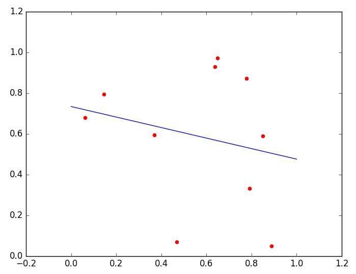
Fig.2: Linear Regression Example Visualization Plot.

Of course, in the context of machine learning, data instances of unknown response variable values would then be placed on the regression line based on their predictor variables, which constitutes predictive power.

Linear regression is an incredibly powerful prediction tool, and is one of the most widely used algorithms available to data scientists.

Related:

• Decision Tree Classifiers: A Concise Technical Overview
• Frequent Pattern Mining and the Apriori Algorithm: A Concise Technical Overview
• Support Vector Machines: A Concise Technical Overview