The Amazing Power of Word Vectors
A fantastic overview of several now-classic papers on word2vec, the work of Mikolov et al. at Google on efficient vector representations of words, and what you can do with them.
Learning word vectors
Mikolov et al. weren’t the first to use continuous vector representations of words, but they did show how to reduce the computational complexity of learning such representations – making it practical to learn high dimensional word vectors on a large amount of data. For example, “We have used a Google News corpus for training the word vectors. This corpus contains about 6B tokens. We have restricted the vocabulary size to the 1 million most frequent words…”
The complexity in neural network language models (feedforward or recurrent) comes from the non-linear hidden layer(s).
While this is what makes neural networks so attractive, we decided to explore simpler models that might not be able to represent the data as precisely as neural networks, but can posssible be trained on much more data efficiently.
Two new architectures are proposed: a Continuous Bag-of-Words model, and aContinuous Skip-gram model. Let’s look at the continuous bag-of-words (CBOW) model first.
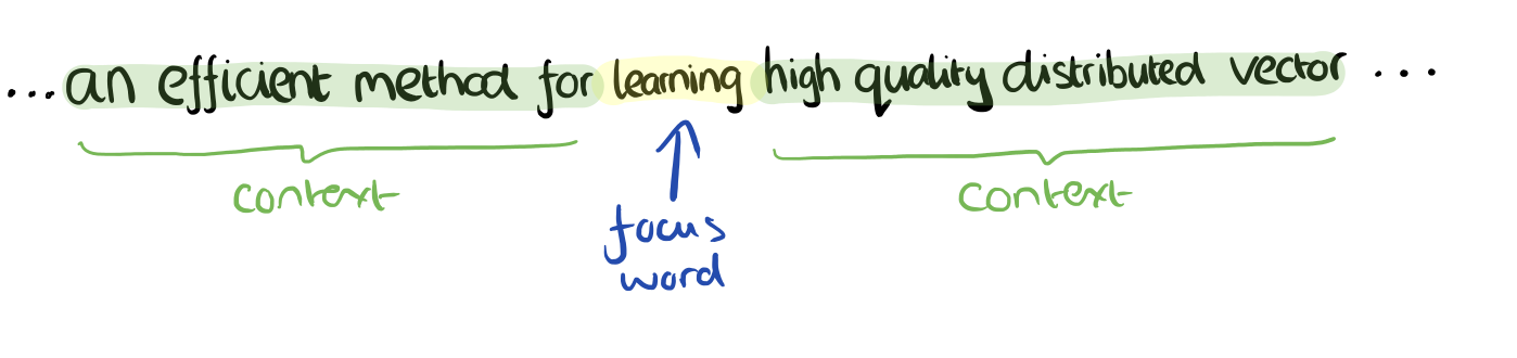
Consider a piece of prose such as “The recently introduced continuous Skip-gram model is an efficient method for learning high-quality distributed vector representations that capture a large number of precises syntatic and semantic word relationships.” Imagine a sliding window over the text, that includes the central word currently in focus, together with the four words and precede it, and the four words that follow it:
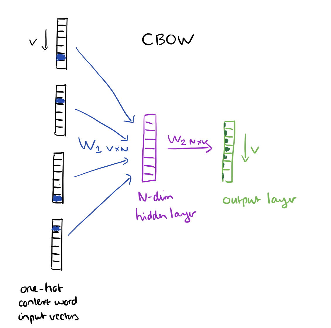
The context words form the input layer. Each word is encoded in one-hot form, so if the vocabulary size is V these will be V-dimensional vectors with just one of the elements set to one, and the rest all zeros. There is a single hidden layer and an output layer.
The training objective is to maximize the conditional probability of observing the actual output word (the focus word) given the input context words, with regard to the weights. In our example, given the input (“an”, “efficient”, “method”, “for”, “high”, “quality”, “distributed”, “vector”) we want to maximize the probability of getting “learning” as the output.
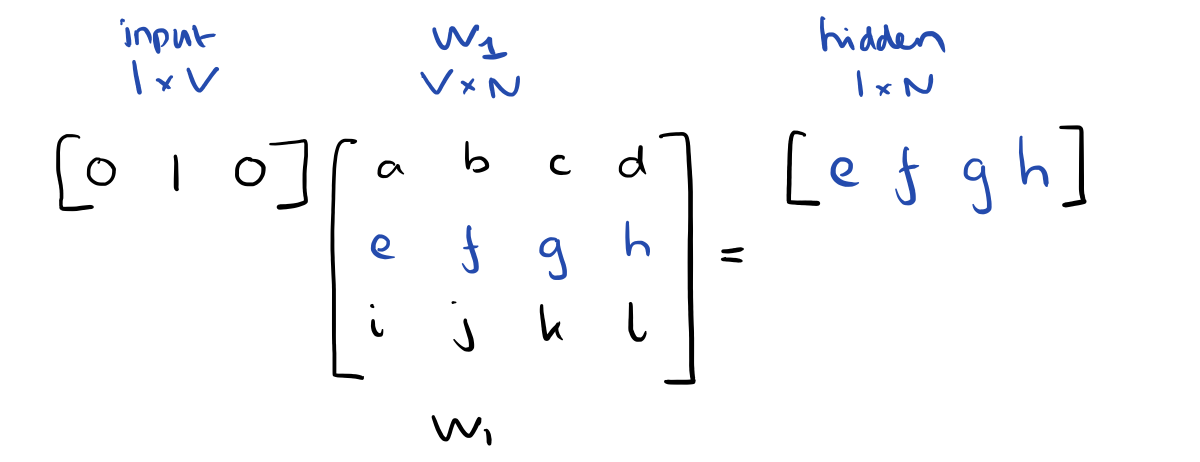
Since our input vectors are one-hot, multiplying an input vector by the weight matrix W1 amounts to simply selecting a row from W1.
Given C input word vectors, the activation function for the hidden layer h amounts to simply summing the corresponding ‘hot’ rows in W1, and dividing by C to take their average.
This implies that the link (activation) function of the hidden layer units is simply linear (i.e., directly passing its weighted sum of inputs to the next layer).
From the hidden layer to the output layer, the second weight matrix W2 can be used to compute a score for each word in the vocabulary, and softmax can be used to obtain the posterior distribution of words.
The skip-gram model is the opposite of the CBOW model. It is constructed with the focus word as the single input vector, and the target context words are now at the output layer:
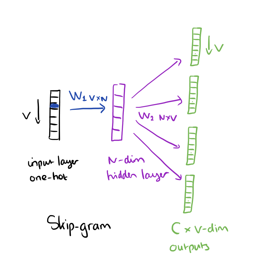
The activation function for the hidden layer simply amounts to copying the corresponding row from the weights matrix W1 (linear) as we saw before. At the output layer, we now output C multinomial distributions instead of just one. The training objective is to mimimize the summed prediction error across all context words in the output layer. In our example, the input would be “learning”, and we hope to see (“an”, “efficient”, “method”, “for”, “high”, “quality”, “distributed”, “vector”) at the output layer.
Optimisations
Having to update every output word vector for every word in a training instance is very expensive...
To solve this problem, an intuition is to limit the number of output vectors that must be updated per training instance. One elegant approach to achieving this is hierarchical softmax; another approach is through sampling.
Hierarchical softmax uses a binary tree to represent all words in the vocabulary. The words themselves are leaves in the tree. For each leaf, there exists a unique path from the root to the leaf, and this path is used to estimate the probability of the word represented by the leaf. “We define this probability as the probability of a random walk starting from the root ending at the leaf in question.”
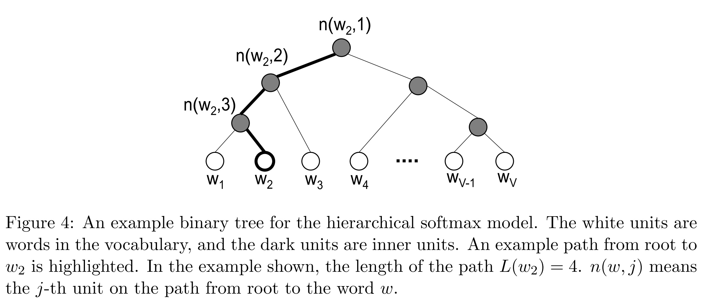
The main advantage is that instead of evaluating V output nodes in the neural network to obtain the probability distribution, it is needed to evaluate only about log2(V) words… In our work we use a binary Huffman tree, as it assigns short codes to the frequent words which results in fast training.
Negative Sampling is simply the idea that we only update a sample of output words per iteration. The target output word should be kept in the sample and gets updated, and we add to this a few (non-target) words as negative samples. “A probabilistic distribution is needed for the sampling process, and it can be arbitrarily chosen… One can determine a good distribution empirically.”
Milokov et al. also use a simple subsampling approach to counter the imbalance between rare and frequent words in the training set (for example, “in”, “the”, and “a” provide less information value than rare words). Each word in the training set is discarded with probability P(wi) where
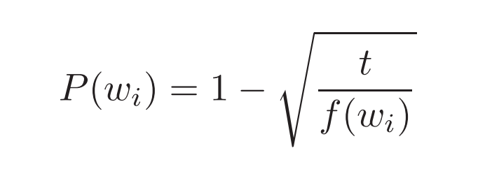
f(wi is the frequency of word wi and t is a chosen threshold, typically around 10-5.
Bio: Adrian Colyer was CTO of SpringSource, then CTO for Apps at VMware and subsequently Pivotal. He is now a Venture Partner at Accel Partners in London, working with early stage and startup companies across Europe. If you’re working on an interesting technology-related business he would love to hear from you: you can reach him at acolyer at accel dot com.
Original. Reposted with permission.
Related: