Artificial Neural Networks (ANN) Introduction, Part 2
Matching the performance of a human brain is a difficult feat, but techniques have been developed to improve the performance of neural network algorithms, 3 of which are discussed in this post: Distortion, mini-batch gradient descent, and dropout.
By Kenneth Soo, Stanford.
We’ve learned how Artificial Neural Networks (ANN) can be used to recognize handwritten digits in a previous post. In the current post, we discuss additional techniques to improve the accuracy of neural networks. Neural networks have been used successfully to solve problems such as image/audio recognition and language processing (see Figure 1).

Figure 1. Uses of neural networks – click to enlarge.
Despite their potential, neural networks were popular only in recent years due to 3 reasons:
Advances in storing and sharing data. With more data available to train on, the performance of neural networks have improved.
Increased computing power. Used mainly to display computer images in the past, graphics processing units (GPUs) were discovered to be up to 150 faster than central processing units (CPUs). Now, GPUs enable neural network models to train efficiently on large datasets.
Enhanced neural network algorithms. Matching the performance of a human brain is a difficult feat, but techniques have been developed to improve the performance of neural network algorithms, 3 of which are discussed in this post:
- Distortion (to increase training data)
- Mini-Batch Gradient Descent (to shorten training time)
- Dropout (to improve prediction accuracy)
Technique 1: Distortion (Increase Training Data)
An artificial neural network learns to recognize handwritten digits when it is given more handwritten images to train on, along with labels of those images. Hence, providing a sufficiently large training dataset of labelled images is critical. However, sometimes the number of available labelled images could be limited.
One way to overcome data shortage is to create more data. By applying different distortions to existing images, each distorted image could be treated as a new training example, thus vastly expanding the size of our training data.

Figure 2. Different distortions applied to the digit “3”. Source: CodeProject
The most effective distortions are the ones that are represented in the existing dataset. For example, we could rotate the images to simulate how people write at an angle. Another technique is elastic deformation, which stretches and squeezes an image at certain points to simulate uncontrolled oscillations of hand muscles (see Figure 2).
Distortion techniques could also be applied to non-visual data. To train a neural network to recognize speech, background noises could be added to existing audio clips to generate new audio samples. Background noises used should already be present in our dataset.
Technique 2: Mini-batch Gradient Descent (Shorten Training Time)
In our previous tutorial, we learned that an artificial neural network comprises neurons, and their activation is governed by a set of rules. Using a mathematical concept called gradient descent, neuron activation rules are tweaked incrementally to improve overall prediction accuracy. To do this however, the neural network cycles through every single training example before determining how best to revise the rules. Hence, while a larger training dataset improves prediction, it will also increase the time taken to process all the training examples. A more efficient solution would be to look at only a small batch of examples each time to approximate the best rule change. This technique is called mini-batch gradient descent.
To understand how this works, let’s look at the following analogy (corresponding technical terms are in bold):
Imagine you are a ruler of a rich kingdom, and you need to decide how much money to allocate (neurons’ rules) to each government department (neurons). Being a rich ruler, you have an unlimited budget, and you want to take into account the wishes of everyone (training data) in your kingdom. However, everyone has a different idea of how the budget should be allocated.
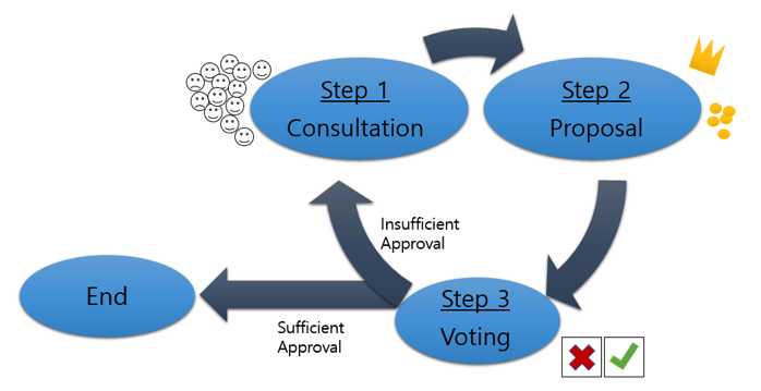
Step 1: You consult individuals on your budget plans. During the interview, each person will state, vaguely, the degree of change (gradient) they want to see in budget allocation. For example, to increase education spending by a bit, and to cut welfare spending by a lot.
Step 2: You take an average of everyone’s views (gradient descent) and revise your budget accordingly (back propagation). Because of your citizens’ ambiguous wordings, you are careful not to change the budget too drastically. Instead, you stick to small changes (learning rate).
Step 3: You present your budget plan, and your citizens vote on whether they approve or disapprove of it (model accuracy).
If you decide that the approval rate is high enough, the budget is passed. Otherwise, you repeat Steps 1 to 3, gradually improving approval rates.
This process is slow because you take one step only after speaking to everyone. One way to speed things up is to approximate the overall opinion by consulting a small subset of your citizens (mini-batch gradient descent).
The following graphs compare prediction accuracy between a vanilla gradient descent (left) vs. mini-batch gradient descent (right):

Using a vanilla gradient descent, prediction error decreased steadily and stabilized after about 250 cycles. On the other hand, a mini-batch gradient descent caused error to decrease with fluctuations and it stabilized only after about 400 cycles. While mini-batch gradient descent needed more cycles to reach the end, each phase cycle was much shorter and thus required less time on the whole.
Technique 3: Dropout (Improve Prediction Accuracy)
Sometimes a neural network might attempt to adjust its neuron activation rules to fit training examples, to the point where the rules do not generalize well to new examples. This phenomenon is called overfitting, a common problem in machine learning which could lead to poor accuracy when predicting new data. The dropout technique could prevent that.
Let’s look at another analogy to describe the intuition behind dropout.
Imagine yourself as the manager of a soccer team. You have two players who have developed strong teamwork and chemistry after playing together for many months. While this is advantageous when both players in the game, their over-reliance on each other might impair performance when one player injured. To overcome this problem, you could force these two players to train with other team members more often.
In the same way, neurons in a neural network might grow reliant on each other when a few neurons co-adapt to patterns in training examples, causing their rules to change in a similar way during gradient descent. Because they do not work with other neurons, they might overlook intrinsic features of training examples, resulting in less robust predictions for new data. To solve this, we could force different neurons to work together by randomly dropping half the neurons in each cycle of a gradient descent.

Neurons which are dropped are completely deactivated and do not send any signals. Hence, they do not affect the activation of neurons in the next layer. Furthermore, their rules remain constant during that cycle, and the entire neural network trains as if these neurons did not exist. The dropout technique thus forces neurons to discover more features in training examples as neurons collaborate in different combinations.
Conclusion
This wraps up the 3 techniques that could be used to improve the accuracy of artificial neural networks. Did you learn something useful today? We would be glad to inform you when we have new tutorials, so that your learning continues!
Sign up below to get bite-sized tutorials delivered to your inbox:

Bio: Kenneth Soo was the top student in the University of Warwick for all 3 years as a math/statistics undergraduate, and is completing his MS in Statistics at Stanford University.
Original. Reposted with permission.
For more posts like this, visit: algobeans.com.
Related: