Artificial Neural Networks (ANN) Introduction, Part 1
This intro to ANNs will look at how we can train an algorithm to recognize images of handwritten digits. We will be using the images from the famous MNIST (Mixed National Institute of Standards and Technology) database.
By Kenneth Soo, Stanford.
Take a look at the picture below and try to identify what it is:

One should be able to tell that it is a giraffe, despite it being strangely fat. We recognize images and objects instantly, even if these images are presented in a form that is different from what we have seen before. We do this with the 80 billion neurons in our brain working together to transmit information. This remarkable system of neurons is also the inspiration behind a widely-used machine learning technique called Artificial Neural Networks (ANN). Some computers using this technique have even out-performed humans in recognizing images.
The Problem
Image recognition is important for many of the advanced technologies we use today. It is used in visual surveillance, guiding autonomous vehicles and even identifying ailments from X-ray images. Most modern smartphones also come with image recognition apps that convert handwriting into typed words.
In this chapter we will look at how we can train an ANN algorithm to recognize images of handwritten digits. We will be using the images from the famous MNIST (Mixed National Institute of Standards and Technology) database.

An Illustration
In this section, we present the performance of an ANN model in recognizing handwritten digits, before explaining how the model works in the next section.
An ANN model is trained by giving it examples of 10,000 handwritten digits, together with the correct digits they represent. This allows the ANN model to understand how the handwriting translates into actual digits. After the ANN model is trained, we can test how well the model performs by giving it 1,000 new handwritten digits without the correct answer. The model is then required to recognize the actual digit.
At the start, the ANN translates handwritten images into pixels – a language it understands. Black pixels are given the value “0” and white pixels the value “1”. Each pixel in an image is called a variable.
Out of the 1,000 handwritten images that the model was asked to recognize, it correctly identified 922 of them, which is a 92.2% accuracy. We can use a contingency table to view the results, as shown below:

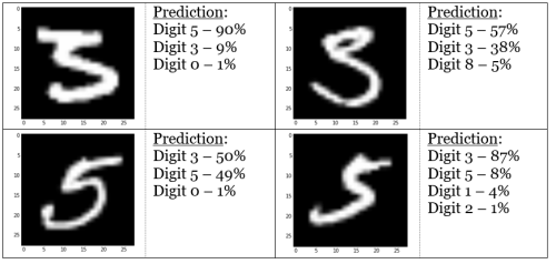
From the table, we can see that when given a handwritten image of either “0” or “1”, the model almost always identifies it correctly. On the other hand, the digit “5” is the trickiest to identify. An advantage of using a contingency table is that it tells us the frequency of mis-identification. Image of the digit “2” are misidentified as “7” or “8” about 8% of the time. Let’s take an in-depth look at some of these misidentified digits:

While the images may look obviously like a digit “2” to human eyes, the ANN is sometimes unable to recognize certain features of images, like the tail of the digit “2” (explained in Limitations section). Another interesting observation is how the model confuses digits “3” and “5” about 10% of the time:
The Neurons That Inspired the Network
Our brain has a large network of interlinked neurons, which act as a highway for information to be transmitted from point A to point B. When different information is sent from A to B, the brain activates different sets of neurons, and so essentially uses a different route to get from A to B. This is how a typical neuron looks like:

At each neuron, dendrites receive incoming signals sent by other neurons. If the neuron receives a high enough level of signals within a certain period of time, the neuron sends an electrical pulse into the terminals. These outgoing signals are then received by other neurons.
Technical Explanation I: How The Model Works
Similarly, in the ANN model, we have an input node, which is the image we give the model, and an output node, which is the digit that the model recognizes. The main characteristics of an ANN model is as such:
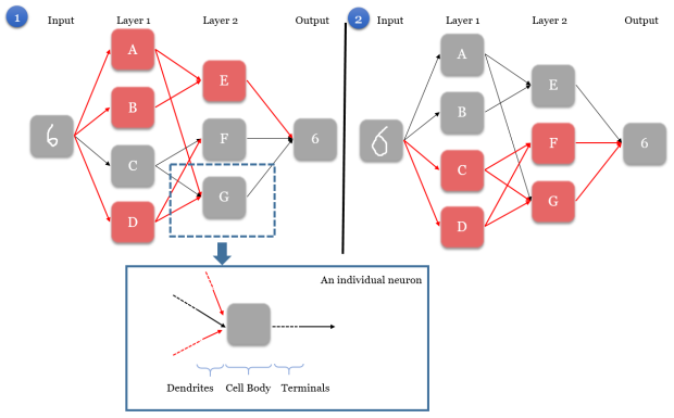
Step 1. When the input node is given an image, it activates a unique set of neurons in the first layer, starting a chain reaction that would pave a unique path to the output node. In Scenario 1, neurons A, B, and D are activated in layer 1.
Step 2. The activated neurons send signals to every connected neuron in the next layer. This directly affects which neurons are activated in the next layer. In Scenario 1, neuron A sends a signal to E and G, neuron B sends a signal to E, and neuron D sends a signal to F and G.
Step 3. In the next layer, each neuron is governed by a rule on what combinations of received signals would activate the neuron. In Scenario 1, neuron E is activated by the signals from A and B. However, for neuron F and G, their neurons’ rules tell them that they have not received the right signals to be activated, and hence they remain grey.
Step 4. Steps 2-3 are repeated for all the remaining layers (it is possible for the model to have more than 2 layers), until we are left with the output node.
Step 5. The output node deduces the correct digit based on signals received from neurons in the layer directly preceding it (layer 2). Each combination of activated neurons in layer 2 leads to one solution, though each solution can be represented by different combinations of activated neurons. In Scenarios 1 & 2, two images are fed as input. Because the images are different, the network activates different neural paths from input to the output. However, the output is still recognizes both images as the digit “6”.
Technical Explanation II: Training The Model
We need to first decide the number of layers and number of neurons in each layer for our ANN model. While there is no limit, a good start is to use 3 layers, with the number of neurons being proportional to the number of variables. For the digit recognizer ANN, we used 3 layers with 500 neurons each. The two key factors involved in training a model are:
- A metric to evaluate the model’s accuracy
- Rules that govern whether neurons are activated or not
A common metric to evaluate model accuracy is the sum of the squared errors (SSE). Put simply, a squared error denotes how close a predicted digit is to the actual digit. The ANN model will try to minimize the SSE by changing the rules that govern neuron activation, and these changes are determined by a mathematical concept known as differentiation.
Each neuron’s rule has two components – the weight (i.e. strength) of incoming signals [w], and the minimum received signal strength required for activation [m]. In the following example, we illustrate the rules for neuron G. Zero weight is given to the signals from A and B (i.e. no connection), and weights of 1, 2, and -1 are given to the signals from C, D, and E respectively. The m-value for G is 2, so G is activated if:
- D is activated and E is not activated, or if,
- C and D are activated.

Limitations
Computationally Expensive. Training an ANN model takes more time and CPU power compared to training other types of models (e.g. random forests). Moreover, the performance of ANN models may not necessarily be superior. Although ANN is not a new technique, it has only been used more frequently in recent years because of hardware advances that made its computing feasible. However, ANN is the basis for more advanced models, like Deep Neural Networks (DNN) which were used by Google in Oct 2015 and Mar 2016 to defeat human champions in the game of Go, widely viewed as an unsolved “grand challenge” for Artificial Intelligence.
Lack of feature recognition. The ANN is unable to recognize images if they take on slight variations in shape, or are placed in a different location. For example, if we want our ANN model to recognize images of cats, and suppose our training examples always feature cats at the bottom of the image, then the ANN model would not recognize the same cats if they appear at the top, or the same cats of larger sizes. An advanced version of ANN called Convolutional Neural Networks (CNN) solves this problem by looking at various regions of the image. In fact, CNNs are also more efficient, and are widely used in image and video recognition. For more information, check out a previous post on Introduction to Convolutional Neural Network.
Additional Notes For Advanced Readers
[This section is intended for readers who have mathematics or computer science background and wish to implement their own ANN.]
The neuron’s rule described in the technical explanation is a mathematical function called “activation function”. It gives zero output when the input is low, and gives positive output when the input is sufficiently high. Commonly-used activation functions include the sigmoid function and rectifier function. The output node is also governed by a function, and softmax (a generalization of the logistic function) is usually used. As such, the ANN can be viewed as “a grand function of functions”. This is also why we use differentiation to find the correct weights through gradient descent. Lastly, note that it is essential to normalize the input data during implementation.
Try out ANN: C++ code by Ben Graham:
github.com/btgraham/Batchwise-Dropout
or Python code by Michael Nielsen:
github.com/mnielsen/neural-networks-and-deep-learning
Did you learn something useful today? We would be glad to inform you when we have new tutorials, so that your learning continues!
Sign up below to get bite-sized tutorials delivered to your inbox:

Bio: Kenneth Soo was the top student in the University of Warwick for all 3 years as a math/statistics undergraduate, and is completing his MS in Statistics at Stanford University.
Original. Reposted with permission.
For more posts like this, visit: algobeans.com.
Related: