 Top 10 Machine Learning Algorithms for Beginners
 Top 10 Machine Learning Algorithms for Beginners
A beginner's introduction to the Top 10 Machine Learning (ML) algorithms, complete with figures and examples for easy understanding.

I. Introduction
The study of ML algorithms has gained immense traction post the Harvard Business Review article terming a ‘Data Scientist’ as the ‘Sexiest job of the 21st century’. So, for those starting out in the field of ML, we decided to do a reboot of our immensely popular Gold blog The 10 Algorithms Machine Learning Engineers need to know - albeit this post is targetted towards beginners.
ML algorithms are those that can learn from data and improve from experience, without human intervention. Learning tasks may include learning the function that maps the input to the output, learning the hidden structure in unlabeled data; or ‘instance-based learning’, where a class label is produced for a new instance by comparing the new instance (row) to instances from the training data, which were stored in memory. ‘Instance-based learning’ does not create an abstraction from specific instances.
II. Types of ML algorithms
There are 3 types of ML algorithms:
1. Supervised learning:
Supervised learning can be explained as follows: use labeled training data to learn the mapping function from the input variables (X) to the output variable (Y).
Y = f (X)
Supervised learning problems can be of two types:
a. Classification: To predict the outcome of a given sample where the output variable is in the form of categories. Examples include labels such as male and female, sick and healthy.
b. Regression: To predict the outcome of a given sample where the output variable is in the form of real values. Examples include real-valued labels denoting the amount of rainfall, the height of a person.
The 1st 5 algorithms that we cover in this blog– Linear Regression, Logistic Regression, CART, Naïve Bayes, KNN are examples of supervised learning.
Ensembling is a type of supervised learning. It means combining the predictions of multiple different weak ML models to predict on a new sample. Algorithms 9-10 that we cover– Bagging with Random Forests, Boosting with XGBoost are examples of ensemble techniques.
2. Unsupervised learning:
Unsupervised learning problems possess only the input variables (X) but no corresponding output variables. It uses unlabeled training data to model the underlying structure of the data.
Unsupervised learning problems can be of two types:
a. Association: To discover the probability of the co-occurrence of items in a collection. It is extensively used in market-basket analysis. Example: If a customer purchases bread, he is 80% likely to also purchase eggs.
b. Clustering: To group samples such that objects within the same cluster are more similar to each other than to the objects from another cluster.
c. Dimensionality Reduction: True to its name, Dimensionality Reduction means reducing the number of variables of a dataset while ensuring that important information is still conveyed. Dimensionality Reduction can be done using Feature Extraction methods and Feature Selection methods. Feature Selection selects a subset of the original variables. Feature Extraction performs data transformation from a high-dimensional space to a low-dimensional space. Example: PCA algorithm is a Feature Extraction approach.
Algorithms 6-8 that we cover here - Apriori, K-means, PCA are examples of unsupervised learning.
3. Reinforcement learning:
Reinforcement learning is a type of machine learning algorithm that allows the agent to decide the best next action based on its current state, by learning behaviours that will maximize the reward.
Reinforcement algorithms usually learn optimal actions through trial and error. They are typically used in robotics – where a robot can learn to avoid collisions by receiving negative feedback after bumping into obstacles, and in video games – where trial and error reveals specific movements that can shoot up a player’s rewards. The agent can then use these rewards to understand the optimal state of game play and choose the next action.
III. Quantifying the popularity of ML algorithms
Survey papers such as these have quantified the 10 most popular data mining algorithms. However, such lists are subjective and as in the case of the quoted paper, the sample size of the polled participants is very narrow and consists of advanced practitioners of data mining. The persons polled were the winners of the ACM KDD Innovation Award, the IEEE ICDM Research Contributions Award; the Program Committee members of the KDD-06, ICDM’06 and SDM’06; and the 145 attendees of the ICDM’06.
The Top 10 algorithms in this blog are meant for beginners and are primarily those that I learnt from the ‘Data Warehousing and Mining’ (DWM) course during my Bachelor’s degree in Computer Engineering at the University of Mumbai. The DWM course is a great introduction to the field of ML algorithms. I have especially included the last 2 algorithms (ensemble methods) based on their prevalence to win Kaggle competitions . Hope you enjoy the article!
IV. Supervised learning algorithms
1. Linear Regression
In ML, we have a set of input variables (x) that are used to determine the output variable (y). A relationship exists between the input variables and the output variable. The goal of ML is to quantify this relationship.
Figure 1: Linear Regression is represented as a line in the form of y = a + bx. Source
Figure 1 shows the plotted x and y values for a dataset. The goal is to fit a line that is nearest to most of the points. This would reduce the distance (‘error’) between the y value of a data point and the line.
2. Logistic Regression
Linear regression predictions are continuous values (rainfall in cm),logistic regression predictions are discrete values (whether a student passed/failed) after applying a transformation function.
Logistic regression is best suited for binary classification (datasets where y = 0 or 1, where 1 denotes the default class. Example: In predicting whether an event will occur or not, the event that it occurs is classified as 1. In predicting whether a person will be sick or not, the sick instances are denoted as 1). It is named after the transformation function used in it, called the logistic function h(x)= 1/ (1 + e^x), which is an S-shaped curve.
In logistic regression, the output is in the form of probabilities of the default class (unlike linear regression, where the output is directly produced). As it is a probability, the output lies in the range of 0-1. The output (y-value) is generated by log transforming the x-value, using the logistic function h(x)= 1/ (1 + e^ -x) . A threshold is then applied to force this probability into a binary classification.
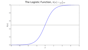
Figure 2: Logistic Regression to determine if a tumour is malignant or benign. Classified as malignant if the probability h(x)>= 0.5. Source
The logistic regression equation P(x) = e ^ (b0 +b1*x) / (1 + e^(b0 + b1*x)) can be transformed into ln(p(x) / 1-p(x)) = b0 + b1*x.
The goal of logistic regression is to use the training data to find the values of coefficients b0 and b1 such that it will minimize the error between the predicted outcome and the actual outcome. These coefficients are estimated using the technique of Maximum Likelihood Estimation.
3. CART
Classification and Regression Trees (CART) is an implementation of Decision Trees, among others such as ID3, C4.5.
The non-terminal nodes are the root node and the internal node. The terminal nodes are the leaf nodes. Each non-terminal node represents a single input variable (x) and a splitting point on that variable; the leaf nodes represent the output variable (y). The model is used as follows to make predictions: walk the splits of the tree to arrive at a leaf node and output the value present at the leaf node.
The decision tree in Figure3 classifies whether a person will buy a sports car or a minivan depending on their age and marital status. If the person is over 30 years and is not married, we walk the tree as follows : ‘over 30 years?’ -> yes -> ’married?’ -> no. Hence, the model outputs a sportscar.
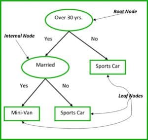
Figure 3: Parts of a decision tree. Source
4. Naïve Bayes
To calculate the probability that an event will occur, given that another event has already occurred, we use Bayes’ Theorem. To calculate the probability of an outcome given the value of some variable, that is, to calculate the probability of a hypothesis(h) being true, given our prior knowledge(d), we use Bayes’ Theorem as follows:
P(h|d)= (P(d|h) * P(h)) / P(d)
where
- P(h|d) = Posterior probability. The probability of hypothesis h being true, given the data d, where P(h|d)= P(d1| h)* P(d2| h)*....*P(dn| h)* P(d)
- P(d|h) = Likelihood. The probability of data d given that the hypothesis h was true.
- P(h) = Class prior probability. The probability of hypothesis h being true (irrespective of the data)
- P(d) = Predictor prior probability. Probability of the data (irrespective of the hypothesis)
This algorithm is called ‘naive’ because it assumes that all the variables are independent of each other, which is a naive assumption to make in real-world examples.
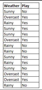
Figure 4: Using Naive Bayes to predict the status of ‘play’ using the variable ‘weather’.
To determine the outcome play= ‘yes’ or ‘no’ given the value of variable weather=’sunny’, calculate P(yes|sunny) and P(no|sunny) and choose the outcome with higher probability.
->P(yes|sunny)= (P(sunny|yes) * P(yes)) / P(sunny)
= (3/9 * 9/14 ) / (5/14)
= 0.60
-> P(no|sunny)= (P(sunny|no) * P(no)) / P(sunny)
= (2/5 * 5/14 ) / (5/14)
= 0.40
Thus, if the weather =’sunny’, the outcome is play= ‘yes’.
5. KNN
The k-nearest neighbours algorithm uses the entire dataset as the training set, rather than splitting the dataset into a trainingset and testset.
When an outcome is required for a new data instance, the KNN algorithm goes through the entire dataset to find the k-nearest instances to the new instance, or the k number of instances most similar to the new record, and then outputs the mean of the outcomes (for a regression problem) or the mode (most frequent class) for a classification problem. The value of k is user-specified.
The similarity between instances is calculated using measures such as Euclidean distance and Hamming distance.