Top 10 Machine Learning Algorithms for Beginners

V. Unsupervised learning algorithms:

6. Apriori

The Apriori algorithm is used in a transactional database to mine frequent itemsets and then generate association rules. It is popularly used in market basket analysis, where one checks for combinations of products that frequently co-occur in the database. In general, we write the association rule for ‘if a person purchases item X, then he purchases item Y’ as : X -> Y.

Example: if a person purchases milk and sugar, then he is likely to purchase coffee powder. This could be written in the form of an association rule as: {milk,sugar} -> coffee powder. Association rules are generated after crossing the threshold for support and confidence.

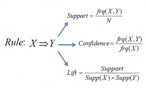
Figure 5: Formulae for support, confidence and lift for the association rule X->Y. SourceThe Support measure helps prune the number of candidate itemsets to be considered during frequent itemset generation. This support measure is guided by the Apriori principle. The Apriori principle states that if an itemset is frequent, then all of its subsets must also be frequent.

7. K-means

K-means is an iterative algorithm that groups similar data into clusters.It calculates the centroids of k clusters and assigns a data point to that cluster having least distance between its centroid and the data point.

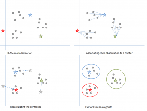
Figure 6: Steps of the K-means algorithm. SourceStep 1: k-means initialization:

a) Choose a value of k. Here, let us take k=3.

b) Randomly assign each data point to any of the 3 clusters.

c) Compute cluster centroid for each of the clusters. The red, blue and green stars denote the centroids for each of the 3 clusters.

Step 2: Associating each observation to a cluster:

Reassign each point to the closest cluster centroid. Here, the upper 5 points got assigned to the cluster with the blue colour centroid. Follow the same procedure to assign points to the clusters containing the red and green colour centroid.

Step 3: Recalculating the centroids:

Calculate the centroids for the new clusters. The old centroids are shown by gray stars while the new centroids are the red, green and blue stars.

Step 4: Iterate, then exit if unchanged.

Repeat steps 2-3 until there is no switching of points from one cluster to another. Once there is no switching for 2 consecutive steps, exit the k-means algorithm.

8. PCA

Principal Component Analysis (PCA) is used to make data easy to explore and visualize by reducing the number of variables. This is done by capturing the maximum variance in the data into a new co-ordinate system with axes called ‘principal components’. Each component is a linear combination of the original variables and is orthogonal to one another. Orthogonality between components indicates that the correlation between these components is zero.

The first principal component captures the direction of the maximum variability in the data. The second principal component captures the remaining variance in the data but has variables uncorrelated with the first component. Similarly, all successive principal components (PC3, PC4 and so on) capture the remaining variance while being uncorrelated with the previous component.

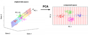
Figure 7: The 3 original variables (genes) are reduced to 2 new variables termed principal components (PC's). Source 

VI. Ensemble learning techniques:

Ensembling means combining the results of multiple learners (classifiers) for improved results, by voting or averaging. Voting is used during classification and averaging is used during regression. The idea is that ensembles of learners perform better than single learners.

There are 3 types of ensembling algorithms: Bagging, Boosting and Stacking. We are not going to cover ‘stacking’ here, but if you’d like a detailed explanation of it, let me know in the comments section below, and I can write a separate blog on it.

9. Bagging with Random Forests

Random Forest (multiple learners) is an improvement over bagged decision trees (a single learner).

Bagging: The first step in bagging is to create multiple models with datasets created using the Bootstrap Sampling method. In Bootstrap Sampling, each generated trainingset is composed of random subsamples from the original dataset. Each of these trainingsets is of the same size as the original dataset, but some records repeat multiple times and some records do not appear at all. Then, the entire original dataset is used as the testset. Thus, if the size of the original dataset is N, then the size of each generated trainingset is also N, with the number of unique records being about (2N/3); the size of the testset is also N.

The second step in bagging is to create multiple models by using the same algorithm on the different generated trainingsets. In this case, let us discuss Random Forest. Unlike a decision tree, where each node is split on the best feature that minimizes error, in random forests, we choose a random selection of features for constructing the best split. The reason for randomness is: even with bagging, when decision trees choose a best feature to split on, they end up with similar structure and correlated predictions. But bagging after splitting on a random subset of features means less correlation among predictions from subtrees.

The number of features to be searched at each split point is specified as a parameter to the random forest algorithm.

Thus, in bagging with Random Forest, each tree is constructed using a random sample of records and each split is constructed using a random sample of predictors.

10. Boosting with AdaBoost

a) Bagging is a parallel ensemble because each model is built independently. On the other hand, boosting is a sequential ensemble where each model is built based on correcting the misclassifications of the previous model.

b) Bagging mostly involves ‘simple voting’, where each classifier votes to obtain a final outcome– one that is determined by the majority of the parallel models; boosting involves ‘weighted voting’, where each classifier votes to obtain a final outcome which is determined by the majority– but the sequential models were built by assigning greater weights to misclassified instances of the previous models.

Adaboost stands for Adaptive Boosting.

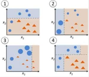
Figure 9: Adaboost for a decision tree. SourceIn Figure 9, steps 1, 2, 3 involve a weak learner called a decision stump (a 1-level decision tree making a prediction based on the value of only 1 input feature; a decision tree with its root immediately connected to its leaves). The process of constructing weak learners continues until a user-defined number of weak learners has been constructed or until there is no further improvement while training. Step 4 combines the 3 decision stumps of the previous models (and thus has 3 splitting rules in the decision tree).

Step 1: Start with 1 decision tree stump to make a decision on 1 input variable:

The size of the data points show that we have applied equal weights to classify them as a circle or triangle. The decision stump has generated a horizontal line in the top half to classify these points. We can see that there are 2 circles incorrectly predicted as triangles. Hence, we will assign higher weights to these 2 circles and apply another decision stump.

Step 2: Move to another decision tree stump to make a decision on another input variable:

We observe that the size of the 2 misclassified circles from the previous step is larger than the remaining points. Now, the 2^nd decision stump will try to predict these 2 circles correctly.

As a result of assigning higher weights, these 2 circles have been correctly classified by the vertical line on the left. But this has now resulted in misclassifying the 3 circles at the top. Hence, we will assign higher weights to these 3 circles at the top and apply another decision stump.

Step 3: Train another decision tree stump to make a decision on another input variable.

The 3 misclassified circles from the previous step are larger than the rest of the data points. Now, a vertical line to the right has been generated to classify the circles and triangles.

Step 4: Combine the decision stumps:

We have combined the separators from the 3 previous models and observe that the complex rule from this model classifies data points correctly as compared to any of the individual weak learners.

 

VII. Conclusion:

To recap, we have learnt:

1. 5 supervised learning techniques- Linear Regression, Logistic Regression, CART, Naïve Bayes, KNN.
2. 3 unsupervised learning techniques- Apriori, K-means, PCA.
3. 2 ensembling techniques- Bagging with Random Forests, Boosting with XGBoost.

In my next blog, we will learn about a technique that has become a rage at Kaggle competitions - the XGBoost algorithm.

Related:

• Top Algorithms and Methods used by Data Scientists
• The 10 Algorithms Machine Learning Engineers need to know
• Top 10 Data Mining Algorithms, Explained