 Machine Learning Algorithms: Which One to Choose for Your Problem
 Machine Learning Algorithms: Which One to Choose for Your Problem
This article will try to explain basic concepts and give some intuition of using different kinds of machine learning algorithms in different tasks. At the end of the article, you’ll find the structured overview of the main features of described algorithms.
By Daniil Korbut, Statsbot.
When I was beginning my way in data science, I often faced the problem of choosing the most appropriate algorithm for my specific problem. If you’re like me, when you open some article about machine learning algorithms, you see dozens of detailed descriptions. The paradox is that they don’t ease the choice.
In this article for Statsbot, I will try to explain basic concepts and give some intuition of using different kinds of machine learning algorithms in different tasks. At the end of the article, you’ll find the structured overview of the main features of described algorithms.

First of all, you should distinguish 4 types of Machine Learning tasks:
- Supervised learning
- Unsupervised learning
- Semi-supervised learning
- Reinforcement learning
Supervised learning
Supervised learning is the task of inferring a function from labeled training data. By fitting to the labeled training set, we want to find the most optimal model parameters to predict unknown labels on other objects (test set). If the label is a real number, we call the task regression. If the label is from the limited number of values, where these values are unordered, then it’s classification.

Illustration source
In unsupervised learning we have less information about objects, in particular, the train set is unlabeled. What is our goal now? It’s possible to observe some similarities between groups of objects and include them in appropriate clusters. Some objects can differ hugely from all clusters, in this way we assume these objects to be anomalies.

Illustration source
Semi-supervised learning tasks include both problems we described earlier: they use labeled and unlabeled data. That is a great opportunity for those who can’t afford labeling their data. The method allows us to significantly improve accuracy, because we can use unlabeled data in the train set with a small amount of labeled data.

Illustration source
Reinforcement learning is not like any of our previous tasks because we don’t have labeled or unlabeled datasets here. RL is an area of machine learning concerned with how software agents ought to take actions in some environment to maximize some notion of cumulative reward.
Illustration source
Commonly used Machine Learning algorithms
Now that we have some intuition about types of machine learning tasks, let’s explore the most popular algorithms with their applications in real life.
Linear Regression and Linear Classifier
These are probably the simplest algorithms in machine learning. You have features x1,...xn of objects (matrix A) and labels (vector b). Your goal is to find the most optimal weights w1,…wn and bias for these features according to some loss function, for example, MSE or MAE for a regression problem. In the case of MSE there is a mathematical equation from the least squares method:
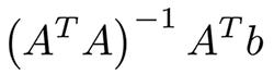
In practice, it’s easier to optimize it with gradient descent, that is much more computationally efficient. Despite the simplicity of this algorithm, it works pretty well when you have thousands of features, for example, bag of words or n-gramms in text analysis. More complex algorithms suffer from overfitting many features and not huge datasets, while linear regression provides decent quality.
Illustration source
Logistic regression
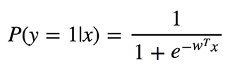
Don’t confuse these classification algorithms with regression methods for using “regression” in its title. Logistic regression performs binary classification, so the label outputs are binary. Let’s define P(y=1|x) as the conditional probability that the output y is 1 under the condition that there is given the input feature vector x. The coefficients w are the weights that the model wants to learn.
Since this algorithm calculates the probability of belonging to each class, you should take into account how much the probability differs from 0 or 1 and average it over all objects as we did with linear regression. Such loss function is the average of cross-entropies:

Don’t panic, I’ll make it easy for you. Allow y to be the right answers: 0 or 1, y_pred — predicted answers. If y equals 0, then the first addend under sum equals 0 and the second is the less the closer our predicted y_pred to 0 according to the properties of the logarithm. Similarly, in the case when yequals 1.
What is great about a logistic regression? It takes linear combination of features and applies non-linear function (sigmoid) to it, so it’s a very very small instance of neural network!
Decision trees
Another popular and easy to understand algorithm is decision trees. Their graphics help you see what you’re thinking and their engine requires a systematic, documented thought process.
The idea of this algorithm is quite simple. In every node we choose the best split among all features and all possible split points. Each split is selected in such a way as to maximize some functional. In classification trees we use cross entropy and Gini index. In regression trees we minimize the sum of a squared error between the predictive variable of the target values of the points that fall in that region and the one we assign to it.

Illustration source
K-means
Sometimes you don’t know any labels and your goal is to assign labels according to the features of objects. This is called clusterization task.
Suppose you want to divide all data-objects into k clusters. You need to select random k points from your data and name them centers of clusters. The clusters of other objects are defined by the closest cluster center. Then, centers of the clusters are converted and the process repeats until convergence.
This is the most clear clusterization technique, which still has some disadvantages. First of all, you should know the amount of clusters that we can’t know. Secondly, the result depends on the points randomly chosen at the beginning and the algorithm doesn’t guarantee that we’ll achieve the global minimum of the functional.
There are a range of clustering methods with different advantages and disadvantages, which you could learn in recommended reading.
Principal component analysis (PCA)
Have you ever prepared for a difficult exam on the last night or during the last hours? You have no chance to remember all the information, but you want to maximize information that you can remember in the time available, for example, learning first the theorems that occur in many exam tickets and so on.
Principal component analysis is based on the same idea. This algorithm provides dimensionality reduction. Sometimes you have a wide range of features, probably highly correlated between each other, and models can easily overfit on a huge amount of data. Then, you can apply PCA.
You should calculate the projection on some vectors to maximize the variance of your data and lose as little information as possible. Surprisingly, these vectors are eigenvectors of correlation matrix of features from a dataset.
Illustration source
- We calculate the correlation matrix of feature columns and find eigenvectors of this matrix.
- We take these multidimensional vectors and calculate the projection of all features on them.
New features are coordinates from a projection and their number depends on the count of eigenvectors, on which you calculate the projection.
Neural networks
I have already mentioned neural networks, when we talked about logistic regression. There are a lot of different architectures that are valuable in very specific tasks. More often, it’s a range of layers or components with linear connections among them and following nonlinearities.
If you’re working with images, convolutional deep neural networks show the great results. Nonlinearities are represented by convolutional and pooling layers, capable of capturing the characteristic features of images.
Illustration source
Conclusion
I hope that I could explain to you common perceptions of the most used machine learning algorithms and give intuition on how to choose one for your specific problem. To make things easier for you, I’ve prepared the structured overview of their main features.
Linear regression and Linear classifier. Despite an apparent simplicity, they are very useful on a huge amount of features where better algorithms suffer from overfitting.
Logistic regression is the simplest non-linear classifier with a linear combination of parameters and nonlinear function (sigmoid) for binary classification.
Decision trees is often similar to people’s decision process and is easy to interpret. But they are most often used in compositions such as Random forest or Gradient boosting.
K-means is more primal, but a very easy to understand algorithm, that can be perfect as a baseline in a variety of problems.
PCA is a great choice to reduce dimensionality of your feature space with minimum loss of information.
Neural Networks are a new era of machine learning algorithms and can be applied for many tasks, but their training needs huge computational complexity.
Recommended sources
- Overview of clustering methods
- A Complete Tutorial on Ridge and Lasso Regression in Python
- YouTube channel about AI for beginners with great tutorials and examples
Bio: Daniil Korbut is a Junior Data Scientist at Statsbot.
Original. Reposted with permission.
Related: