Understanding Learning Rates and How It Improves Performance in Deep Learning
Furthermore, the learning rate affects how quickly our model can converge to a local minima (aka arrive at the best accuracy). Thus getting it right from the get go would mean lesser time for us to train the model.
By Hafidz Zulkifli, Data Scientist at Seek
This post is an attempt to document my understanding on the following topic:
- What is the learning rate? What is it’s significance?
- How does one systematically arrive at a good learning rate?
- Why do we change the learning rate during training?
- How do we deal with learning rates when using pretrained model?
Much of this post are based on the stuff written by past fast.ai fellows [1], [2], [5] and [3] . This is a concise version of it, arranged in a way for one to quickly get to the meat of the material. Do go over the references for more details.
First off, what is a learning rate?
Learning rate is a hyper-parameter that controls how much we are adjusting the weights of our network with respect the loss gradient. The lower the value, the slower we travel along the downward slope. While this might be a good idea (using a low learning rate) in terms of making sure that we do not miss any local minima, it could also mean that we’ll be taking a long time to converge — especially if we get stuck on a plateau region.
The following formula shows the relationship.
new_weight = existing_weight — learning_rate * gradient
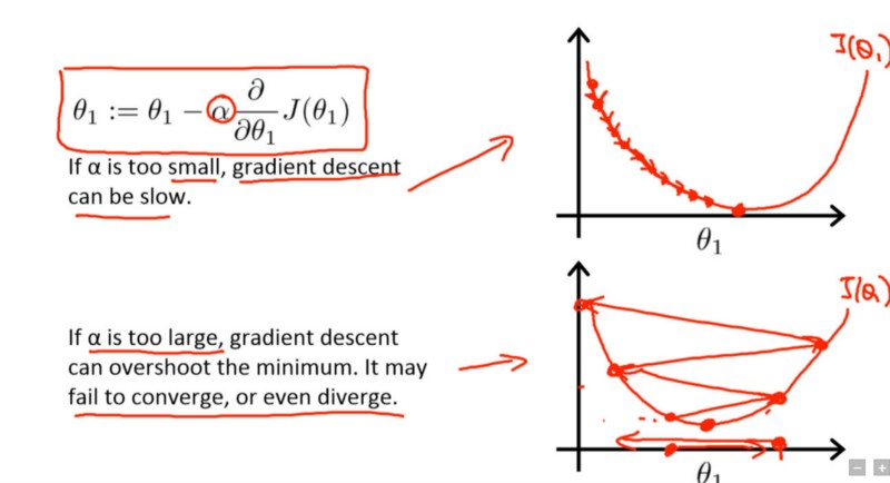
Gradient descent with small (top) and large (bottom) learning rates. Source: Andrew Ng’s Machine Learning course on Coursera
Typically learning rates are configured naively at random by the user. At best, the user would leverage on past experiences (or other types of learning material) to gain the intuition on what is the best value to use in setting learning rates.
As such, it’s often hard to get it right. The below diagram demonstrates the different scenarios one can fall into when configuring the learning rate.
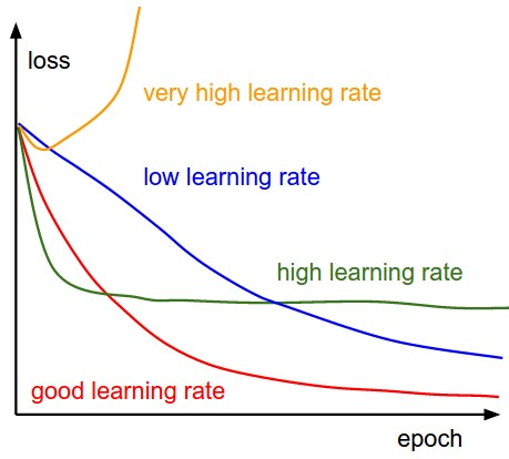
Effect of various learning rates on convergence (Img Credit: cs231n)
Furthermore, the learning rate affects how quickly our model can converge to a local minima (aka arrive at the best accuracy). Thus getting it right from the get go would mean lesser time for us to train the model.
Less training time, lesser money spent on GPU cloud compute. :)
Is there a better way to determine the learning rate?
In Section 3.3 of “Cyclical Learning Rates for Training Neural Networks.” [4], Leslie N. Smith argued that you could estimate a good learning rate by training the model initially with a very low learning rate and increasing it (either linearly or exponentially) at each iteration.
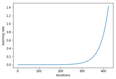
Learning rate increases after each mini-batch
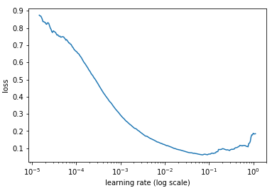
If we record the learning at each iteration and plot the learning rate (log) against loss; we will see that as the learning rate increase, there will be a point where the loss stops decreasing and starts to increase. In practice, our learning rate should ideally be somewhere to the left to the lowest point of the graph (as demonstrated in below graph). In this case, 0.001 to 0.01.
The above seems useful. How can I start using it?
At the moment it is supported as a function in the fast.ai package, developed by Jeremy Howard as a way to abstract the pytorch package (much like how Keras is an abstraction for Tensorflow).
One only needs to type in the following command to start finding the most optimal learning rate to use before training a neural network.
Making It Better
At this juncture we’ve covered what learning rate is all about, it’s importance, and how can we systematically come to an optimal value to use when we start training our model.
Next we would go through how learning rates can still be used to improve our model’s performance.
The conventional wisdom
Typically when one sets their learning rate and trains the model, one would only wait for the learning rate to decrease over time and for the model to eventually converge.
However, as the gradient reaches a plateau, the training loss becomes harder to improve. In [3], Dauphin et al argue that the difficulty in minimizing the loss arises from saddle points rather than poor local minima.
A saddle point in the error surface. A saddle point is a point where derivatives of the function become zero but the point is not a local extremum on all axes. (Img Credit: safaribooksonline)
So how do we escape from this?
There are a few options that we could consider. In general, taking a quote from [1],
… instead of using a fixed value for learning rate and decreasing it over time, if the training doesn’t improve our loss anymore, we’re going to be changing the learning rate every iteration according to some cyclic function f. Each cycle has a fixed length in terms of number of iterations. This method lets the learning rate cyclically vary between reasonable boundary values. It helps because, if we get stuck on saddle points, increasing the learning rate allows more rapid traversal of saddle point plateaus.
In [2], Leslie proposes a ‘triangular’ method where the learning rates are restarted after every few iterations.
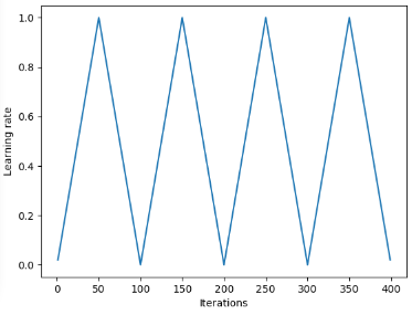
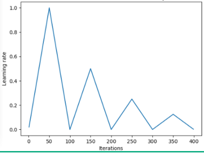
‘Triangular’ and ‘Triangular2’ methods for cycling learning rate proposed by Leslie N. Smith. On the left plot min and max lr are kept the same. On the right the difference is cut in half after each cycle.
Another method that is also popular is called Stochastic Gradient Descent with Warm Restarts, proposed by Loshchilov & Hutter [6]. This method basically uses the cosine function as the cyclic function and restarts the learning rate at the maximum at each cycle. The “warm” bit comes from the fact that when the learning rate is restarted, it does not start from scratch; but rather from the parameters to which the model converged during the last step [7].
While there are variations of this, the below diagram demonstrates one of its implementation, where each cycle is set to the same time period.
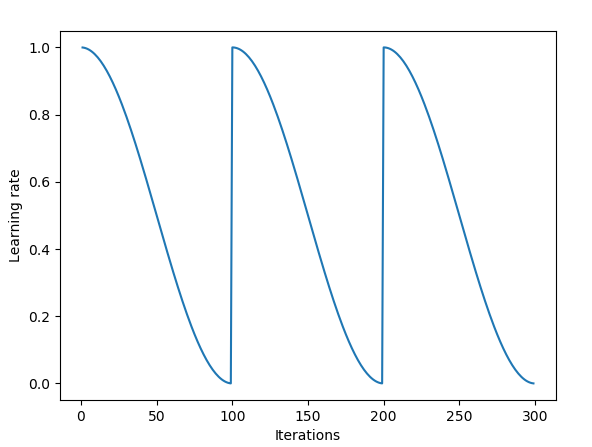
SGDR plot, learning rate vs iteration.
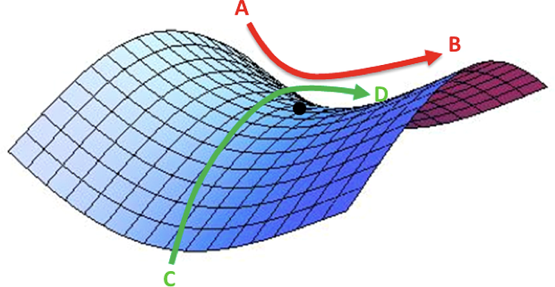
Thus we now have a way to reduce the training time, by basically periodically jumping around “mountains” (below).
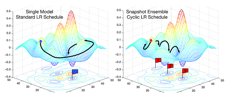
Comparing fixed LR and Cyclic LR (image by ruder.io)
Aside from saving time, research also shows that using these method tend to improve classification accuracy without tuning and within fewer iteration.
Learning Rate in Transfer Learning
In the fast.ai course, much emphasis is given in leveraging pretrained model when solving AI problems. For example, in solving an image classification problem, students are taught how to use pretrained models such VGG or Resnet50 and connecting it to whatever image dataset that you want to predict.
To summarize how model building is done in fast.ai (the program, not to be confused with the fast.ai package), below are the few steps [8] that we’d normally take:
1. Enable data augmentation, and precompute=True
2. Uselr_find()to find highest learning rate where loss is still clearly improving
3. Train last layer from precomputed activations for 1–2 epochs
4. Train last layer with data augmentation (i.e. precompute=False) for 2–3 epochs with cycle_len=1
5. Unfreeze all layers
6. Set earlier layers to 3x-10x lower learning rate than next higher layer
7. Uselr_find()again
8. Train full network with cycle_mult=2 until over-fitting
From the steps above, we notice that step 2, 5, and 7 are concerned about learning rate. In the earlier part of this post, we’ve basically covered item no.2 of the steps mentioned — where we touched on how to derive the best learning rate prior to training the model.
In the subsequent section we went over how by using SGDR we are able to reduce the training time and increase accuracy by restarting the learning rate every now and then to avoid regions where gradient close to zero.
In this last section, we’ll go over differential learning, and how it’s being used to determine the learning rate when training models attached with a pretrained model.
What is differential learning?
It is a method where you set different learning rates to different layers in the network during training. This is in contrast to how people normally configure the learning rate, which is to use the same rate throughout the network during training.
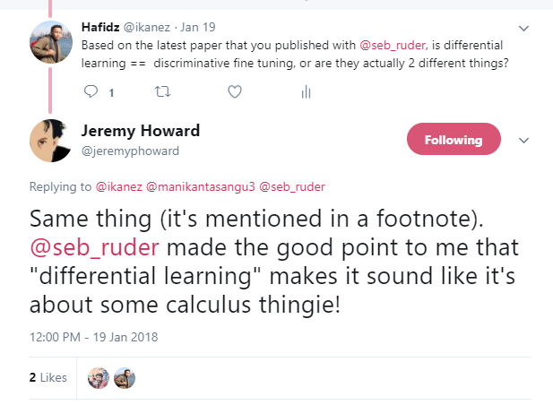
One reason why I just love Twitter — direct answer from the man himself.
While writing this post, Jeremy published a paper with Sebastian Ruder [9] which dives deeper into this topic. So I guess differential learning rates has a new name now — discriminative fine tuning. :)
To illustrate the concept a bit clearer, we can refer to the below diagram, where a pretrained model is split into 3 groups, where each group would be configured with an increasing learning rate value.
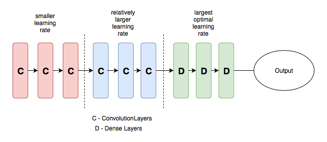
Sample CNN with differential learning rate. Image credit from [3]
The intuition behind this method of configuration is that the first few layers would typically contain very granular details of the data, such as the lines and the edges — of which we normally wouldn’t want to change much and like to retain it’s information. As such, there’s not much need to change their weights by a big amount.
In contrast, in later layers such as the ones in green above — where we get detailed features of the data such as eyeballs or mouth or nose; we might not necessarily need to keep them.
How does this compare with other methods of fine tuning?
In [9], it is argued that fine-tuning an entire model would be too costly as some could have more than 100 layers. As such, what people usually do is to fine-tune the model one layer at a time.
However, this introduces a sequential requirement, hindering parallelism, and requires multiple passes through the dataset, resulting in overfitting for small datasets.
It has also been demonstrated that the methods introduced in [9] are able to improve both accuracy and reduce error rates in various NLP classification tasks (below)
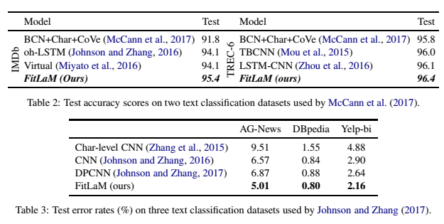
Results taken from [9]
References:
[1] Improving the way we work with learning rate.
[2] The Cyclical Learning Rate technique.
[3] Transfer Learning using differential learning rates.
[4] Leslie N. Smith. Cyclical Learning Rates for Training Neural Networks.
[5] Estimating an Optimal Learning Rate for a Deep Neural Network
[6] Stochastic Gradient Descent with Warm Restarts
[7] Optimization for Deep Learning Highlights in 2017
[8] Lesson 1 Notebook, fast.ai Part 1 V2
[9] Fine-tuned Language Models for Text Classification
Bio: Hafidz Zulkifli is a Data Scientist at Seek in Malaysia.
Original. Reposted with permission.
Related:
- Is Learning Rate Useful in Artificial Neural Networks?
- Estimating an Optimal Learning Rate For a Deep Neural Network
- TensorFlow: What Parameters to Optimize?