Getting Started with PyTorch Part 1: Understanding How Automatic Differentiation Works
PyTorch has emerged as a major contender in the race to be the king of deep learning frameworks. What makes it really luring is it’s dynamic computation graph paradigm.
By Ayoosh Kathuria, Research Intern
When I started to code neural networks, I ended up using what everyone else around me was using. TensorFlow.
But recently, PyTorch has emerged as a major contender in the race to be the king of deep learning frameworks. What makes it really luring is it’s dynamic computation graph paradigm. Don’t worry if the last line doesn’t make sense to you now. By the end of this post, it will. But take my word that it makes debugging neural networks way easier.
I've been using PyTorch a few months now and I've never felt better. I have more energy. My skin is clearer. My eye sight has improved.
— Andrej Karpathy (@karpathy) May 26, 2017
If you’re wondering why your energy has been low lately, switch to PyTorch!
Prerequisites
Before we begin, I must point out that you should have at least the basic idea about:
- Concepts related to training of neural networks, particularly backpropagation and gradient descent.
- Applying the chain rule to compute derivatives.
- How classes work in Python. (Or a general idea about Object Oriented Programming)
In case, you’re missing any of the above, I’ve provided links at the end of the article to guide you.
So, it’s time to get started with PyTorch. This is the first in a series of tutorials on PyTorch.
This is the part 1 where I’ll describe the basic building blocks, and Autograd.
NOTE: An important thing to notice is that the tutorial is made for PyTorch 0.3 and lower versions. The latest version on offer is 0.4. I’ve decided to stick with 0.3 because as of now, 0.3 is the version that is shipped in Conda and pip channels. Also, most of PyTorch code that is used in open source hasn’t been updated to incorporate some of the changes proposed in 0.4. I, however, will point out at certain places where things differ in 0.3 and 0.4.
Building Block #1 : Tensors
If you’ve ever done machine learning in python, you’ve probably come across NumPy. The reason why we use Numpy is because it’s much faster than Python lists at doing matrix ops. Why? Because it does most of the heavy lifting in C.
But, in case of training deep neural networks, NumPy arrays simply don’t cut it. I’m too lazy to do the actual calculations here (google for “FLOPS in one iteration of ResNet to get an idea), but code utilising NumPy arrays alone would take months to train some of the state of the art networks.
This is where Tensors come into play. PyTorch provides us with a data structure called a Tensor, which is very similar to NumPy’s ndarray. But unlike the latter, tensors can tap into the resources of a GPU to significantly speed up matrix operations.
Here is how you make a Tensor.
In [1]: import torch

In [2]: import numpy as np

In [3]: arr = np.random.randn((3,5))

In [4]: arr

Out[4]:
array([[-1.00034281, -0.07042071,  0.81870386],
       [-0.86401346, -1.4290267 , -1.12398822],
       [-1.14619856,  0.39963316, -1.11038695],
       [ 0.00215314,  0.68790149, -0.55967659]])

In [5]: tens = torch.from_numpy(arr)

In [6]: tens

Out[6]:

-1.0003 -0.0704  0.8187
-0.8640 -1.4290 -1.1240
-1.1462  0.3996 -1.1104
0.0022  0.6879 -0.5597
[torch.DoubleTensor of size 4x3]

In [7]: another_tensor = torch.LongTensor([[2,4],[5,6]])

In [7]: another_tensor

Out[13]:
 2  4
 5  6
[torch.LongTensor of size 2x2]

In [8]: random_tensor = torch.randn((4,3))

In [9]: random_tensor

Out[9]:
1.0070 -0.6404  1.2707
-0.7767  0.1075  0.4539
-0.1782 -0.0091 -1.0463
 0.4164 -1.1172 -0.2888
[torch.FloatTensor of size 4x3]
Building Block #2 : Computation Graph
Now, we are at the business side of things. When a neural network is trained, we need to compute gradients of the loss function, with respect to every weight and bias, and then update these weights using gradient descent.
With neural networks hitting billions of weights, doing the above step efficiently can make or break the feasibility of training.
Building Block #2.1: Computation Graphs
Computation graphs lie at the heart of the way modern deep learning networks work, and PyTorch is no exception. Let us first get the hang of what they are.
Suppose, your model is described like this:
b = w1 * a
c = w2 * a
d = (w3 * b) + (w4 * c)
L = f(d)
If I were to actually draw the computation graph, it would probably look like this.
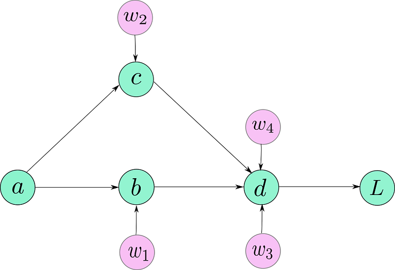
Computation Graph for our Model
NOW, you must note, that the above figure is not entirely an accurate representation of how the graph is represented under the hood by PyTorch. However, for now, it’s enough to drive our point home.
Why should we create such a graph when we can sequentially execute the operations required to compute the output?
Imagine, what were to happen, if you didn’t merely have to calculate the output but also train the network. You’ll have to compute the gradients for all the weights labelled by purple nodes. That would require you to figure your way around chain rule, and then update the weights.
The computation graph is simply a data structure that allows you to efficiently apply the chain rule to compute gradients for all of your parameters.

Applying the chain rule using computation graphs
Here are a couple of things to notice. First, that the directions of the arrows are now reversed in the graph. That’s because we are backpropagating, and arrows marks the flow of gradients backwards.
Second, for the sake of these example, you can think of the gradients I have written as edge weights. Notice, these gradients don’t require chain rule to be computed.
Now, in order to compute the gradient of any node, say, L, with respect of any other node, say c ( dL / dc) all we have to do is.
- Trace the path from L to c. This would be L → d → c.
- Multiply all the edge weights as you traverse along this path. The quantity you end up with is: ( dL / dd ) * ( dd / dc ) = ( dL / dc)
- If there are multiple paths, add their results. For example in case of dL/da, we have two paths. L → d → c → a and L → d → b→ a. We add their contributions to get the gradient of L w.r.t. a.
[( dL / dd ) * ( dd / dc ) * ( dc / da )] + [( dL / dd ) * ( dd / db ) * ( db / da )]
In principle, one could start at L, and start traversing the graph backwards, calculating gradients for every node that comes along the way.