How to calculate confidence intervals for performance metrics in Machine Learning using an automatic bootstrap method
Are your model performance measurements very precise due to a “large” test set, or very uncertain due to a “small” or imbalanced test set?
By David B Rosen (PhD), Lead Data Scientist for Automated Credit Approval at IBM Global Financing
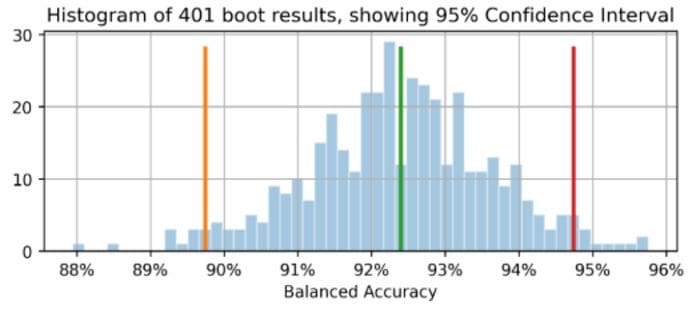
The orange line shows 89.7% as the lower bound of the Balanced Accuracy confidence interval, green for the original observed Balanced Accuracy=92.4% (point estimate), and red for upper bound of 94.7%. (This and all images are by the author unless otherwise noted.)
Introduction
If you report your classifier’s performance as having Accuracy=94.8% and F1=92.3% on a test set, this doesn’t mean much without knowing something about the size and composition of the test set. The margin of error of those performance measurements will vary a lot depending on the size of the test set, or, for an imbalanced dataset, primarily depending on how many independent instances of the minority class it contains (more copies of the same instances from oversampling doesn’t help for this purpose).
If you were able to collect another, independent test set of similar origin, the Accuracy and F1 of your model on this dataset are unlikely to be the same, but how much different might they plausibly be? A question similar to this is answered in statistics as the confidence interval of the measurement.
If we were to draw many independent sample datasets from the underlying population, then for 95% of those datasets, the true underlying population value of the metric would be within the 95% confidence interval that we would calculate for that particular sample dataset.
In this article we will show you how to calculate confidence intervals for any number of Machine Learning performance metrics at once, with a bootstrap method that automatically determines how many boot sample datasets to generate by default.
If you just want to see how to invoke this code to calculate confidence intervals, skip to the section “Calculate the results!” down below.
The bootstrap methodology
If we were able to draw additional test datasets from the true distribution underlying the data, we would be able to see the distribution of the performance metric(s) of interest across those datasets. (When drawing those datasets we would not do anything to prevent drawing an identical or similar instance multiple times, although this might only happen rarely.)
Since we can’t do that, the next best thing is to draw additional datasets from the empirical distribution of this test dataset, which means sampling, with replacement, from its instances to generate new bootstrap sample datasets. Sampling with replacement means once we draw a particular instance, we put it back in so that we might draw it again for the same sample dataset. Therefore, each such dataset generally has multiple copies of some of the instances, and does not include all of the instances that are in the base test set.
If we sampled without replacement, then we would simply get an identical copy of the original dataset every time, shuffled in a different random order, which would not be of any use.
The percentile bootstrap methodology for estimating the confidence interval is as follows:
- Generate
nboots“bootstrap sample” datasets, each the same size as the original test set. Each sample dataset is obtained by drawing instances at random from the test set with replacement. - On each of the sample datasets, calculate the metric and save it.
- The 95% confidence interval is given by the 2.5th to the 97.5th percentile among the
nbootscalculated values of the metric. Ifnboots=1001 and you sorted the values in a series/array/list X of length 1001, the 0th percentile is X[0] and the 100th percentile is X[1000], so the confidence interval would be given by X[25] to X[975].
Of course you can calculate as many metrics as you like for each sample dataset in step 2, but in step 3 you would find the percentiles for each metric separately.
Example Dataset and Confidence Interval Results
We will use results from this prior article as an example: How To Deal With Imbalanced Classification, Without Re-balancing the Data: Before considering oversampling your skewed data, try adjusting your classification decision threshold.
In that article we used the highly-imbalanced two-class Kaggle credit card fraud identification data set. We chose to use a classification threshold quite different from the default 0.5 threshold that is implicit in using the predict() method, making it unnecessary to balance the data. This approach is sometimes termed threshold moving, in which our classifier assigns the class by applying the chosen threshold to the predicted class probability provided by the predict_proba() method.
We will limit the scope of this article (and code) to binary classification: classes 0 and 1, with class 1 by convention being the “positive” class and specifically the minority class for imbalanced data, although the code should work for regression (single continuous target) as well.
Generating one boot sample dataset
Although our confidence interval code can handle various numbers of data arguments to be passed to the metric functions, we will focus on sklearn-style metrics, which always accept two data arguments, y_true and y_pred, where y_pred will be either binary class predictions (0 or 1), or continuous class-probability or decision function predictions, or even continuous regression predictions if y_true is continuous as well. The following function generates a single boot sample dataset. It accepts any data_args but in our case these arguments will be ytest(our actual/true test set target values in the prior article) and hardpredtst_tuned_thresh (the predicted class). Both contain zeros and ones to indicate the true or predicted class for each instance.
Custom metric specificity_score() and utility functions
We will define a custom metric function for Specificity, which is just another name for the Recall of the negative class (class 0). Also a calc_metrics function which which applies a sequence of metrics of interest to our data, and a couple of utility functions for it:
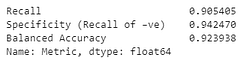
Here we make our list of metrics and apply them to the data. We did not consider Accuracy to be a relevant metric because a false negative (misclassifying a true fraud as legit) is much more costly to the business than a false positive (misclassifying a true legit as a fraud), whereas Accuracy treats both types of misclassification are equally bad and therefore favors correctly-classifying those whose true class is the majority class because these occur much more often and so contribute much more to the overall Accuracy.
met=[ metrics.recall_score, specificity_score,
      metrics.balanced_accuracy_score
    ]
calc_metrics(met, ytest, hardpredtst_tuned_thresh)
Making each boot sample dataset and calculating metrics for it
In raw_metric_samples() we will actually generate multiple sample datasets one by one and save the metrics of each:
You give raw_metric_samples() a list of metrics (or just one metric) of interest as well as the true and predicted class data, and it obtains nboots sample datasets and returns a dataframe with just the metrics’ values calculated from each dataset. Through _boot_generator() it invokes one_boot() one at a time in a generator expression rather than storing all the datasets at once as a potentially-huge list.
Look at metrics on 7 boot sample datasets
We make our list of metric functions and invoke raw_metric_samples() to get the results for just 7 sample datasets. We are invoking raw_metric_samples() here for understanding — it is not necessary in order to get confidence intervals using ci_auto() below, although specifying a list of metrics (or just one metric) for ci_auto() is necessary.
np.random.seed(13)
raw_metric_samples(met, ytest, hardpredtst_tuned_thresh,
          nboots=7).style.format('{:.2%}')  #optional #style
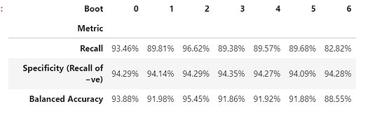
Each column above contains the metrics calculated from one boot sample dataset (numbered 0 to 6), so the calculated metric values vary due to the random sampling.
Number of boot datasets, with calculated default
In our implementation, by default the number of boot datasets nboots will be calculated automatically from the desired confidence level (e.g. 95%) so as to meet the recommendation by North, Curtis, and Sham to have a minimum number of boot results in each tail of the distribution. (Actually this recommendation applies to p-values and thus hypothesis test acceptance regions, but confidence intervals are similar enough to those to use this as a rule of thumb.) Although those authors recommend a minimum of 10 boot results in the tail, Davidson & MacKinnon recommend at least 399 boots for 95% confidence, which requires 11 boots in the tail, so we use this more-conservative recommendation.
We specify alpha which is 1 - confidence level. E.g. 95% confidence becomes 0.95 and alpha=0.05. If you specify an explicit number of boots (perhaps a smaller nboots because you want faster results) but it is not enough for your requested alpha, a higher alpha will be chosen automatically in order to get an accurate confidence interval for that number of boots. A minimum of 51 boots will be used because any less can only accurately calculate bizarrely-small confidence levels (such as 40% confidence which gives an interval from the 30th percentile to the 70th percentile, which has 40% inside the interval but 60% outside it) and it is not clear that the minimum-boots recommendation even contemplated such a case.
The function get_alpha_nboots() sets the default nboots or modifies the requested alpha and nboots per above:
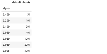
Let’s show the default nboots for various values of alpha:
g = get_alpha_nboots
pd.DataFrame( [ g(0.40), g(0.20, None), g(0.10), g(), g(alpha=0.02),
                g(alpha=0.01, nboots=None), g(0.005, nboots=None)
              ], columns=['alpha', 'default nboots']
            ).set_index('alpha')
Here’s what happens if we request an explicit nboots:
req=[(0.01,3000), (0.01,401), (0.01,2)]
out=[get_alpha_nboots(*args) for args in req]
mydf = lambda x: pd.DataFrame(x, columns=['alpha', 'nboots'])
pd.concat([mydf(req),mydf(out)],axis=1, keys=('Requested','Using'))
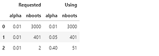
Small nboots values increased alpha to 0.05 and 0.40, and nboots=2 gets changed to the minimum of 51.
Histogram of bootstrap sample datasets showing confidence interval just for Balanced Accuracy
Again we don’t need to do this in order to get the confidence intervals below by invoking ci_auto().
np.random.seed(13)
metric_boot_histogram\
  (metrics.balanced_accuracy_score, ytest, hardpredtst_tuned_thresh)

The orange line shows 89.7% as the lower bound of the Balanced Accuracy confidence interval, green for the original observed Balanced Accuracy=92.4% (point estimate), and red for upper bound of 94.7%. (Same image appears at the top of this article.)
How to calculate all the confidence intervals for list of metrics
Here is the main function that invokes the above and calculates the confidence intervals from the percentiles of the metric results, and inserts the point estimates as the first column of its output dataframe of results.
Calculate the results!
This is all we really needed to do: invoke ci_auto() as follows with a list of metrics (met assigned above) to get their confidence intervals. The percentage formatting is optional:
np.random.seed(13)
ci_auto( met, ytest, hardpredtst_tuned_thresh
       ).style.format('{:.2%}')
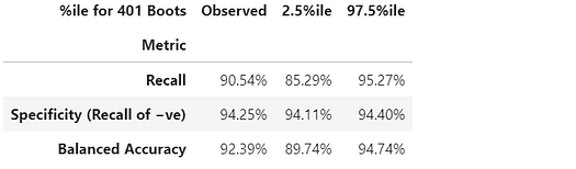
Discussion of resulting confidence intervals
Here’s the confusion matrix from the original article. Class 0 is the negatives (majority class) and Class 1 is the positives (very rare class)
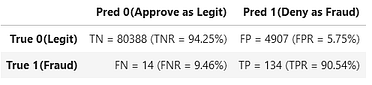
The Recall (True Positive Rate) of 134/(134+14) has the widest confidence interval because this is a binomial proportion involving small counts.
The Specificity (True Negative Rate) is 80,388/(80,388+4,907), which involves much larger counts, so it has an extremely narrow confidence interval of just [94.11% to 94.40%].
Since the Balanced Accuracy is calculated as simply an average of the Recall and the Specificity, the width of its confidence interval is intermediate between theirs’.
Metric measurement imprecision due to variations in test data, vs. variations in train data
Here we have not considered the variability in the model based on the randomness of our training data (although that can also be of interest for some purposes, e.g. if you have automated repeated re-training and want to know how much the performance of future models might vary), but rather only the variability in the measurement of the performance of this particular model (created from some particular training data) due to the randomness of our test data.
If we had enough independent test data, we could measure the performance of this particular model on the underlying population very precisely, and we would know how it will perform if this model is deployed, irrespective of how we built the model and of whether we might obtain a better or worse model with a different training sample dataset.
Independence of individual instances
The bootstrap method assumes that each of your instances (cases, observations) is drawn independently from an underlying population. If your test set has groups of rows that are not independent of each other, for example repeated observations of the same entity that are likely to be correlated with one another, or instances that are oversampled/replicated/generated-from other instances in your test set, the results might not be valid. You might need to use grouped sampling, where you draw entire groups together at random rather than individual rows, while avoiding breaking up any group or just using part of it.
Also you want to make sure you don’t have groups that were split across the training and test set, because then the test set is not necessarily independent and you might get undetected overfitting. For example if you use oversampling you should generally only do only after it has been split from the test set, not before. And normally you would oversample the training set but not the test set, since the test set must remain representative of instances the model will see upon future deployment. And for cross-validation you would want to use scikit-learn’s model_selection.GroupKFold().
Conclusion
You can always calculate confidence intervals for your evaluation metric(s) to see how precisely your test data enables you to measure your model’s performance. I’m planning another article to demonstrate confidence intervals for metrics that evaluate probability predictions (or confidence scores — no relation to statistical confidence), i.e. soft classification, such as Log Loss or ROC AUC, rather than the metrics we used here which evaluate the discrete choice of class by the model (hard classification). The same code works for both, as well as for regression (predicting a continuous target variable) — you just have to pass it a different kind of prediction (and different kind of true targets in the case of regression).
This jupyter notebook is available in github: bootConfIntAutoV1o_standalone.ipynb
Was this article informative and/or useful? Please post a comment below if you have any comments or questions about this article or about confidence intervals, the bootstrap, number of boots, this implementation, dataset, model, threshold moving, or results.
In addition to the aforementioned prior article, you might also be interested in my How to Auto-Detect the Date/Datetime Columns and Set Their Datatype When Reading a CSV File in Pandas, though it’s not directly related to the present article.
Bio: David B Rosen (PhD) is Lead Data Scientist for Automated Credit Approval at IBM Global Financing. Find more of David's writing at dabruro.medium.com.
Original. Reposted with permission.
Related:
- How to do “Limitless” Math in Python
- Advanced Statistical Concepts in Data Science
- How to Determine the Best Fitting Data Distribution Using Python