Implementing Deep Learning Methods and Feature Engineering for Text Data: The Skip-gram Model
Just like we discussed in the CBOW model, we need to model this Skip-gram architecture now as a deep learning classification model such that we take in the target word as our input and try to predict the context words.
Editor's note: This post is only one part of a far more thorough and in-depth original, found here, which covers much more than what is included here.
The Skip-gram Model
The Skip-gram model architecture usually tries to achieve the reverse of what the CBOW model does. It tries to predict the source context words (surrounding words) given a target word (the center word). Considering our simple sentence from earlier, “the quick brown fox jumps over the lazy dog”. If we used the CBOW model, we get pairs of (context_window, target_word)where if we consider a context window of size 2, we have examples like ([quick, fox], brown), ([the, brown], quick), ([the, dog], lazy) and so on. Now considering that the skip-gram model’s aim is to predict the context from the target word, the model typically inverts the contexts and targets, and tries to predict each context word from its target word. Hence the task becomes to predict the context [quick, fox] given target word ‘brown’ or [the, brown] given target word ‘quick’ and so on. Thus the model tries to predict the context_window words based on the target_word.
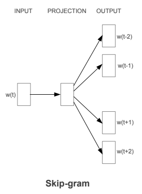
The Skip-gram model architecture (Source: https://arxiv.org/pdf/1301.3781.pdf Mikolov el al.)
Just like we discussed in the CBOW model, we need to model this Skip-gram architecture now as a deep learning classification model such that we take in the target word as our input and try to predict the context words.This becomes slightly complex since we have multiple words in our context. We simplify this further by breaking down each (target, context_words) pair into (target, context) pairs such that each context consists of only one word. Hence our dataset from earlier gets transformed into pairs like (brown, quick), (brown, fox), (quick, the), (quick, brown) and so on. But how to supervise or train the model to know what is contextual and what is not?
For this, we feed our skip-gram model pairs of (X, Y) where X is our input and Y is our label. We do this by using [(target, context), 1] pairs as positive input samples where target is our word of interest and context is a context word occurring near the target word and the positive label 1 indicates this is a contextually relevant pair. We also feed in [(target, random), 0] pairs as negative input samples where target is again our word of interest but random is just a randomly selected word from our vocabulary which has no context or association with our target word. Hence the negative label 0indicates this is a contextually irrelevant pair. We do this so that the model can then learn which pairs of words are contextually relevant and which are not and generate similar embeddings for semantically similar words.
Implementing the Skip-gram Model
Let’s now try and implement this model from scratch to gain some perspective on how things work behind the scenes and also so that we can compare it with our implementation of the CBOW model. We will leverage our Bible corpus as usual which is contained in the norm_bible variable for training our model. The implementation will focus on five parts
- Build the corpus vocabulary
- Build a skip-gram [(target, context), relevancy] generator
- Build the skip-gram model architecture
- Train the Model
- Get Word Embeddings
Let’s get cracking and build our skip-gram Word2Vec model!
Build the corpus vocabulary
To start off, we will follow the standard process of building our corpus vocabulary where we extract out each unique word from our vocabulary and assign a unique identifier, similar to what we did in the CBOW model. We also maintain mappings to transform words to their unique identifiers and vice-versa.
Vocabulary Size: 12425
Vocabulary Sample: [('perceived', 1460), ('flagon', 7287), ('gardener', 11641), ('named', 973), ('remain', 732), ('sticketh', 10622), ('abstinence', 11848), ('rufus', 8190), ('adversary', 2018), ('jehoiachin', 3189)]
Just like we wanted, each unique word from the corpus is a part of our vocabulary now with a unique numeric identifier.
Build a skip-gram [(target, context), relevancy] generator
It’s now time to build out our skip-gram generator which will give us pair of words and their relevance like we discussed earlier. Luckily, keras has a nifty skipgrams utility which can be used and we don’t have to manually implement this generator like we did in CBOW.
Note: The function
skipgrams(…)is present inkeras.preprocessing.sequenceThis function transforms a sequence of word indexes (list of integers) into tuples of words of the form:
- (word, word in the same window), with label 1 (positive samples).
- (word, random word from the vocabulary), with label 0 (negative samples).
(james (1154), king (13)) -> 1
(king (13), james (1154)) -> 1
(james (1154), perform (1249)) -> 0
(bible (5766), dismissed (6274)) -> 0
(king (13), alter (5275)) -> 0
(james (1154), bible (5766)) -> 1
(king (13), bible (5766)) -> 1
(bible (5766), king (13)) -> 1
(king (13), compassion (1279)) -> 0
(james (1154), foreskins (4844)) -> 0
Thus you can see we have successfully generated our required skip-grams and based on the sample skip-grams in the preceding output, you can clearly see what is relevant and what is irrelevant based on the label (0 or 1).
Build the skip-gram model architecture
We now leverage keras on top of tensorflow to build our deep learning architecture for the skip-gram model. For this our inputs will be our target word and context or random word pair. Each of which are passed to an embedding layer (initialized with random weights) of it’s own. Once we obtain the word embeddings for the target and the context word, we pass it to a merge layer where we compute the dot product of these two vectors. Then we pass on this dot product value to a dense sigmoid layer which predicts either a 1 or a 0 depending on if the pair of words are contextually relevant or just random words (Y’). We match this with the actual relevance label (Y), compute the loss by leveraging the mean_squared_error loss and perform backpropagation with each epoch to update the embedding layer in the process. Following code shows us our model architecture.
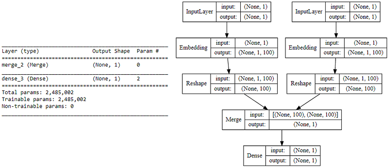
Skip-gram model summary and architecture
Understanding the above deep learning model is pretty straightforward. However, I will try to summarize the core concepts of this model in simple terms for ease of understanding. We have a pair of input words for each training example consisting of one input target word having a unique numeric identifier and one context word having a unique numeric identifier. If it is a positive sample the word has contextual meaning, is a context wordand our label Y=1, else if it is a negative sample, the word has no contextual meaning, is just a random word and our label Y=0. We will pass each of them to an embedding layer of their own, having size (vocab_size x embed_size) which will give us dense word embeddings for each of these two words (1 x embed_size for each word). Next up we use a merge layer to compute the dot product of these two embeddings and get the dot product value. This is then sent to the dense sigmoid layer which outputs either a 1 or 0. We compare this with the actual label Y (1 or 0), compute the loss, backpropagate the errors to adjust the weights (in the embedding layer) and repeat this process for all (target, context) pairs for multiple epochs. The following figure tries to explain the same.
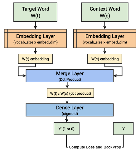
Visual depiction of the Skip-gram deep learning model
Let’s now start training our model with our skip-grams.
Train the Model
Running the model on our complete corpus takes a fair bit of time but lesser than the CBOW model. Hence I just ran it for 5 epochs. You can leverage the following code and increase it for more epochs if necessary.
Epoch: 1 Loss: 4529.63803683
Epoch: 2 Loss: 3750.71884749
Epoch: 3 Loss: 3752.47489296
Epoch: 4 Loss: 3793.9177565
Epoch: 5 Loss: 3716.07605051
Once this model is trained, similar words should have similar weights based off the embedding layer and we can test out the same.
Get Word Embeddings
To get word embeddings for our entire vocabulary, we can extract out the same from our embedding layer by leveraging the following code. Do note that we are only interested in the target word embedding layer, hence we will extract the embeddings from our word_model embedding layer. We don’t take the embedding at position 0 since none of our words in the vocabulary have a numeric identifier of 0 and we ignore it.
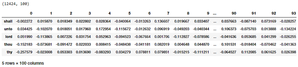
Word Embeddings for our vocabulary based on the Skip-gram model
Thus you can clearly see that each word has a dense embedding of size (1x100) as depicted in the preceding output similar to what we had obtained from the CBOW model. Let’s now apply the euclidean distance metric on these dense embedding vectors to generate a pairwise distance metric for each word in our vocabulary. We can then find out the n-nearest neighbors of each word of interest based on the shortest (euclidean) distance similar to what we did on the embeddings from our CBOW model.
(12424, 12424)

{'egypt': ['pharaoh', 'mighty', 'houses', 'kept', 'possess'],
 'famine': ['rivers', 'foot', 'pestilence', 'wash', 'sabbaths'],
 'god': ['evil', 'iniquity', 'none', 'mighty', 'mercy'],
 'gospel': ['grace', 'shame', 'believed', 'verily', 'everlasting'],
 'jesus': ['christ', 'faith', 'disciples', 'dead', 'say'],
 'john': ['ghost', 'knew', 'peter', 'alone', 'master'],
 'moses': ['commanded', 'offerings', 'kept', 'presence', 'lamb'],
 'noah': ['flood', 'shem', 'peleg', 'abram', 'chose']}
You can clearly see from the results that a lot of the similar words for each of the words of interest are making sense and we have obtained better results as compared to our CBOW model. Let’s visualize these words embeddings now using t-SNE which stands for t-distributed stochastic neighbor embedding a popular dimensionality reduction technique to visualize higher dimension spaces in lower dimensions (e.g. 2-D).
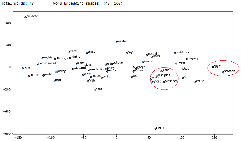
Visualizing skip-gram word2vec word embeddings using t-SNE
I have marked some circles in red which seemed to show different words of contextual similarity positioned near each other in the vector space. If you find any other interesting patterns feel free to let me know!
Bio: Dipanjan Sarkar is a Data Scientist @Intel, an author, a mentor @Springboard, a writer, and a sports and sitcom addict.
Original. Reposted with permission.
Related:
- Text Data Preprocessing: A Walkthrough in Python
- A General Approach to Preprocessing Text Data
- A Framework for Approaching Textual Data Science Tasks