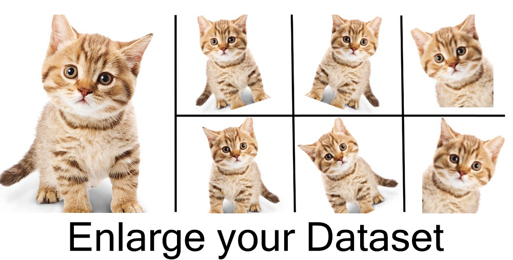
Data Augmentation: How to use Deep Learning when you have Limited Data
This article is a comprehensive review of Data Augmentation techniques for Deep Learning, specific to images.
By Bharath Raj, thatbrguy.
We have all been there. You have a stellar concept that can be implemented using a machine learning model. Feeling ebullient, you open your web browser and search for relevant data. Chances are, you find a dataset that has around a few hundred images.
You recall that most popular datasets have images in the order of tens of thousands (or more). You also recall someone mentioning having a large dataset is crucial for good performance. Feeling disappointed, you wonder; can my “state-of-the-art” neural network perform well with the meagre amount of data I have?
The answer is, yes! But before we get into the magic of making that happen, we need to reflect upon some basic questions.
Why is there a need for a large amount of data?
When you train a machine learning model, what you’re really doing is tuning its parameters such that it can map a particular input (say, an image) to some output (a label). Our optimization goal is to chase that sweet spot where our model’s loss is low, which happens when your parameters are tuned in the right way.
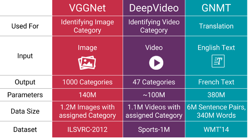
State of the art neural networks typically have parameters in the order of millions!
Naturally, if you have a lot of parameters, you would need to show your machine learning model a proportional amount of examples, to get good performance. Also, the number of parameters you need is proportional to the complexity of the task your model has to perform.
How do I get more data, if I don’t have “more data”?
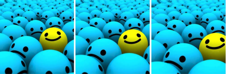
You don’t need to hunt for novel new images that can be added to your dataset. Why? Because, neural networks aren’t smart to begin with. For instance, a poorly trained neural network would think that these three tennis balls shown below, are distinct, unique images.
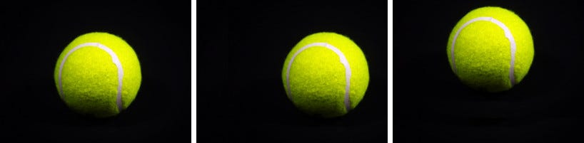
The same tennis ball, but translated.
So, to get more data, we just need to make minor alterations to our existing dataset. Minor changes such as flips or translations or rotations. Our neural network would think these are distinct images anyway.
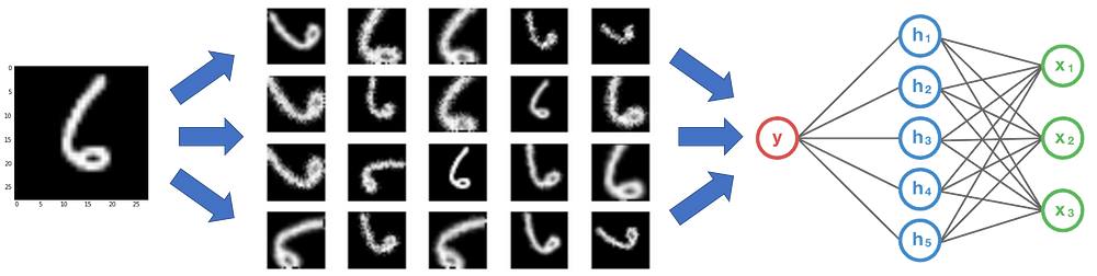
A convolutional neural network that can robustly classify objects even if its placed in different orientations is said to have the property called invariance. More specifically, a CNN can be invariant to translation, viewpoint, size orillumination (Or a combination of the above).
This essentially is the premise of data augmentation. In the real world scenario, we may have a dataset of images taken in a limited set of conditions. But, our target application may exist in a variety of conditions, such as different orientation, location, scale, brightness etc. We account for these situations by training our neural network with additional synthetically modified data.
Can augmentation help even if I have lots of data?
Yes. It can help to increase the amount of relevant data in your dataset. This is related to the way with which neural networks learn. Let me illustrate it with an example.
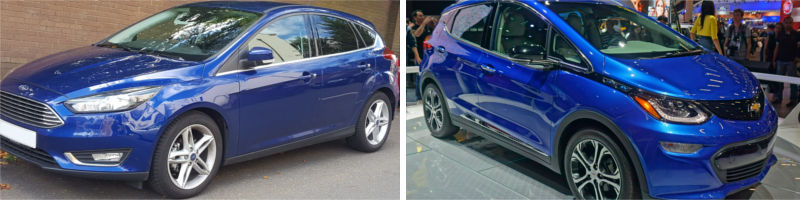
Imagine that you have a dataset, consisting of two brands of cars, as shown above. Let’s assume that all cars of brand A are aligned exactly like the picture in the left (i.e. All cars are facing left) . Likewise, all cars of brand Bare aligned exactly like the picture in the right (i.e. Facing right) . Now, you feed this dataset to your “state-of-the-art” neural network, and you hope to get impressive results once it’s trained.
Let’s say it’s done training, and you feed the image above, which is a Brand A car. But your neural network outputs that it’s a Brand B car! You’re confused. Didn’t you just get a 95% accuracy on your dataset using your “state-of-the-art” neural network? I’m not exaggerating, similar incidents and goof-ups have occurred in the past.
Why does this happen? It happens because that’s how most machine learning algorithms work. It finds the most obvious features that distinguishes one class from another. Here, the feature was that all cars of Brand A were facing left, and all cars of Brand B are facing right.
Your neural network is only as good as the data you feed it.
How do we prevent this happening? We have to reduce the amount of irrelevant features in the dataset. For our car model classifier above, a simple solution would be to add pictures of cars of both classes, facing the other direction to our original dataset. Better yet, you can just flip the images in the existing dataset horizontally such that they face the other side! Now, on training the neural network on this new dataset, you get the performance that you intended to get.
By performing augmentation, can prevent your neural network from learning irrelevant patterns, essentially boosting overall performance.
Getting Started
Before we dive into the various augmentation techniques, there’s one issue that we must consider beforehand.
Where do we augment data in our ML pipeline?
The answer may seem quite obvious; we do augmentation before we feed the data to the model right? Yes, but you have two options here. One option is to perform all the necessary transformations beforehand, essentially increasing the size of your dataset. The other option is to perform these transformations on a mini-batch, just before feeding it to your machine learning model.
The first option is known as offline augmentation. This method is preferred for relatively smaller datasets, as you would end up increasing the size of the dataset by a factor equal to the number of transformations you perform (For example, by flipping all my images, I would increase the size of my dataset by a factor of 2).
The second option is known as online augmentation, or augmentation on the fly. This method is preferred for larger datasets, as you can’t afford the explosive increase in size. Instead, you would perform transformations on the mini-batches that you would feed to your model. Some machine learning frameworks have support for online augmentation, which can be accelerated on the GPU.
Popular Augmentation Techniques
In this section, we present some basic but powerful augmentation techniques that are popularly used. Before we explore these techniques, for simplicity, let us make one assumption. The assumption is that, we don’t need to consider what lies beyond the image’s boundary. We’ll use the below techniques such that our assumption is valid.
What would happen if we use a technique that forces us to guess what lies beyond an image’s boundary? In this case, we need to interpolate some information. We’ll discuss this in detail after we cover the types of augmentation.
For each of these techniques, we also specify the factor by which the size of your dataset would get increased (aka. Data Augmentation Factor).
1. Flip
You can flip images horizontally and vertically. Some frameworks do not provide function for vertical flips. But, a vertical flip is equivalent to rotating an image by 180 degrees and then performing a horizontal flip. Below are examples for images that are flipped.

You can perform flips by using any of the following commands, from your favorite packages. Data Augmentation Factor = 2 to 4x
# NumPy.'img' = A single image.
flip_1 = np.fliplr(img)
# TensorFlow. 'x' = A placeholder for an image.
shape = [height, width, channels]
x = tf.placeholder(dtype = tf.float32, shape = shape)
flip_2 = tf.image.flip_up_down(x)
flip_3 = tf.image.flip_left_right(x)
flip_4 = tf.image.random_flip_up_down(x)
flip_5 = tf.image.random_flip_left_right(x)
2. Rotation
One key thing to note about this operation is that image dimensions may not be preserved after rotation. If your image is a square, rotating it at right angles will preserve the image size. If it’s a rectangle, rotating it by 180 degrees would preserve the size. Rotating the image by finer angles will also change the final image size. We’ll see how we can deal with this issue in the next section. Below are examples of square images rotated at right angles.

You can perform rotations by using any of the following commands, from your favorite packages. Data Augmentation Factor = 2 to 4x
# Placeholders: 'x' = A single image, 'y' = A batch of images
# 'k' denotes the number of 90 degree anticlockwise rotations
shape = [height, width, channels]
x = tf.placeholder(dtype = tf.float32, shape = shape)
rot_90 = tf.image.rot90(img, k=1)
rot_180 = tf.image.rot90(img, k=2)
# To rotate in any angle. In the example below, 'angles' is in radians
shape = [batch, height, width, 3]
y = tf.placeholder(dtype = tf.float32, shape = shape)
rot_tf_180 = tf.contrib.image.rotate(y, angles=3.1415)
# Scikit-Image. 'angle' = Degrees. 'img' = Input Image
# For details about 'mode', checkout the interpolation section below.
rot = skimage.transform.rotate(img, angle=45, mode='reflect')
3. Scale
The image can be scaled outward or inward. While scaling outward, the final image size will be larger than the original image size. Most image frameworks cut out a section from the new image, with size equal to the original image. We’ll deal with scaling inward in the next section, as it reduces the image size, forcing us to make assumptions about what lies beyond the boundary. Below are examples or images being scaled.
You can perform scaling by using the following commands, using scikit-image. Data Augmentation Factor = Arbitrary.
# Scikit Image. 'img' = Input Image, 'scale' = Scale factor
# For details about 'mode', checkout the interpolation section below.
scale_out = skimage.transform.rescale(img, scale=2.0, mode='constant')
scale_in = skimage.transform.rescale(img, scale=0.5, mode='constant')
# Don't forget to crop the images back to the original size (for
# scale_out)
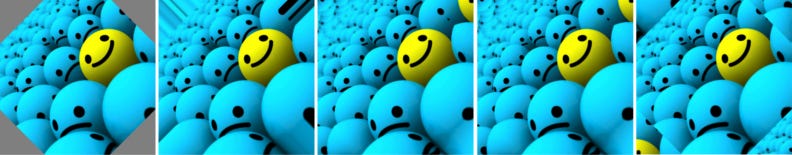
4. Crop
Unlike scaling, we just randomly sample a section from the original image. We then resize this section to the original image size. This method is popularly known as random cropping. Below are examples of random cropping. If you look closely, you can notice the difference between this method and scaling.

You can perform random crops by using any the following command for TensorFlow. Data Augmentation Factor = Arbitrary.
# TensorFlow. 'x' = A placeholder for an image.
original_size = [height, width, channels]
x = tf.placeholder(dtype = tf.float32, shape = original_size)
# Use the following commands to perform random crops
crop_size = [new_height, new_width, channels]
seed = np.random.randint(1234)
x = tf.random_crop(x, size = crop_size, seed = seed)
output = tf.images.resize_images(x, size = original_size)
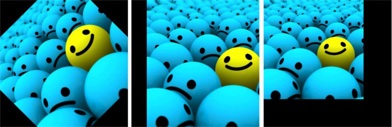
5. Translation
Translation just involves moving the image along the X or Y direction (or both). In the following example, we assume that the image has a black background beyond its boundary, and are translated appropriately. This method of augmentation is very useful as most objects can be located at almost anywhere in the image. This forces your convolutional neural network to look everywhere.
You can perform translations in TensorFlow by using the following commands. Data Augmentation Factor = Arbitrary.
# pad_left, pad_right, pad_top, pad_bottom denote the pixel
# displacement. Set one of them to the desired value and rest to 0
shape = [batch, height, width, channels]
x = tf.placeholder(dtype = tf.float32, shape = shape)
# We use two functions to get our desired augmentation
x = tf.image.pad_to_bounding_box(x, pad_top, pad_left, height + pad_bottom
+ pad_top, width + pad_right + pad_left)
output = tf.image.crop_to_bounding_box(x, pad_bottom, pad_right, height, width)
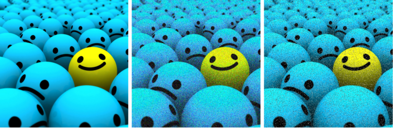
6. Gaussian Noise
Over-fitting usually happens when your neural network tries to learn high frequency features (patterns that occur a lot) that may not be useful. Gaussian noise, which has zero mean, essentially has data points in all frequencies, effectively distorting the high frequency features. This also means that lower frequency components (usually, your intended data) are also distorted, but your neural network can learn to look past that. Adding just the right amount of noise can enhance the learning capability.
A toned down version of this is the salt and pepper noise, which presents itself as random black and white pixels spread through the image. This is similar to the effect produced by adding Gaussian noise to an image, but may have a lower information distortion level.
You can add Gaussian noise to your image by using the following command, on TensorFlow. Data Augmentation Factor = 2x.
#TensorFlow. 'x' = A placeholder for an image.
shape = [height, width, channels]
x = tf.placeholder(dtype = tf.float32, shape = shape)
# Adding Gaussian noise
noise = tf.random_normal(shape=tf.shape(x), mean=0.0, stddev=1.0,
dtype=tf.float32)
output = tf.add(x, noise)
Advanced Augmentation Techniques
Real world, natural data can still exist in a variety of conditions that cannot be accounted for by the above simple methods. For instance, let us take the task of identifying the landscape in photograph. The landscape could be anything: freezing tundras, grasslands, forests and so on. Sounds like a pretty straight forward classification task right? You’d be right, except for one thing. We are overlooking a crucial feature in the photographs that would affect the performance — The season in which the photograph was taken.
If our neural network does not understand the fact that certain landscapes can exist in a variety of conditions (snow, damp, bright etc.), it may spuriously label frozen lakeshores as glaciers or wet fields as swamps.
One way to mitigate this situation is to add more pictures such that we account for all the seasonal changes. But that is an arduous task. Extending our data augmentation concept, imagine how cool it would be to generate effects such as different seasons artificially?
Conditional GANs to the rescue!
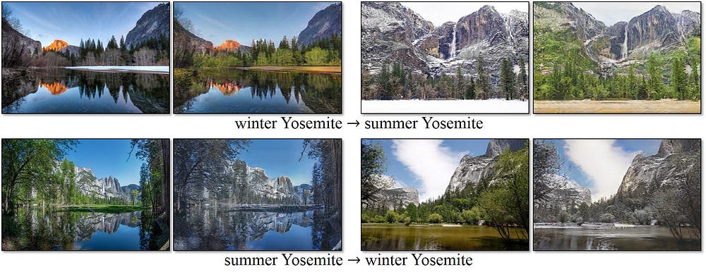
Without going into gory detail, conditional GANs can transform an image from one domain to an image to another domain. If you think it sounds too vague, it’s not; that’s literally how powerful this neural network is! Below is an example of conditional GANs used to transform photographs of summer sceneries to winter sceneries.
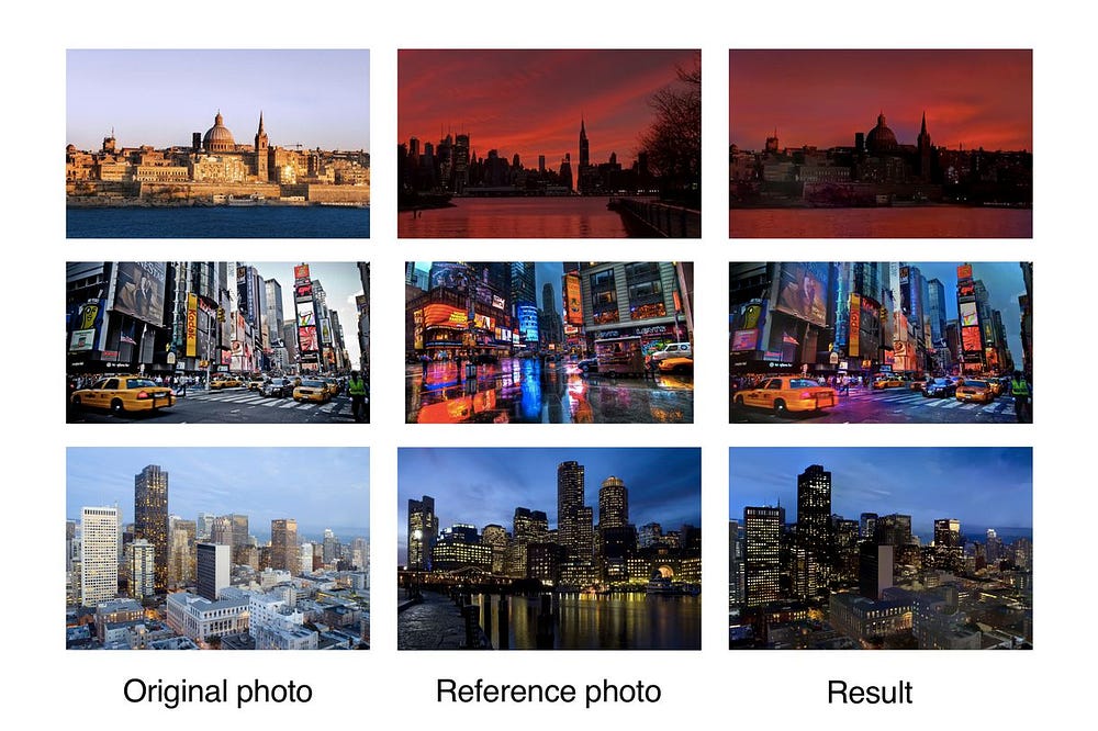
The above method is robust, but computationally intensive. A cheaper alternative would be something called neural style transfer. It grabs the texture/ambiance/appearance of one image (aka, the “style”) and mixes it with the content of another. Using this powerful technique, we produce an effect similar to that of our conditional GAN (In fact, this method was introduced before cGANs were invented!).
The only downside of this method is that, the output tends to looks more artistic rather than realistic. However, there are certain advancements such as Deep Photo Style Transfer, shown below, that have impressive results.
We have not explored these techniques in great depth as we are not concerned with their inner working. We can use existing trained models, along with the magic of transfer learning, to use it for augmentation.
A brief note on interpolation
What if you wanted to translate an image that doesn’t have a black background? What if you wanted to scale inward? Or rotate in finer angles? After we perform these transformations, we need to preserve our original image size. Since our image does not have any information about things outside it’s boundary, we need to make some assumptions. Usually, the space beyond the image’s boundary is assumed to be the constant 0 at every point. Hence, when you do these transformations, you get a black region where the image is not defined.
But is that the right assumption? In the real world scenario, it’s mostly a no. Image processing and ML frameworks have some standard ways with which you can decide on how to fill the unknown space. They are defined as follows.
1. Constant
The simplest interpolation method is to fill the unknown region with some constant value. This may not work for natural images, but can work for images taken in a monochromatic background
2. Edge
The edge values of the image are extended after the boundary. This method can work for mild translations.
3. Reflect
The image pixel values are reflected along the image boundary. This method is useful for continuous or natural backgrounds containing trees, mountains etc.
4. Symmetric
This method is similar to reflect, except for the fact that, at the boundary of reflection, a copy of the edge pixels are made. Normally, reflect and symmetric can be used interchangeably, but differences will be visible while dealing with very small images or patterns.
5. Wrap
The image is just repeated beyond its boundary, as if it’s being tiled. This method is not as popularly used as the rest as it does not make sense for a lot of scenarios.
Besides these, you can design your own methods for dealing with undefined space, but usually these methods would just do fine for most classification problems.
So, if I use ALL of these techniques, my ML algorithm would be robust right?
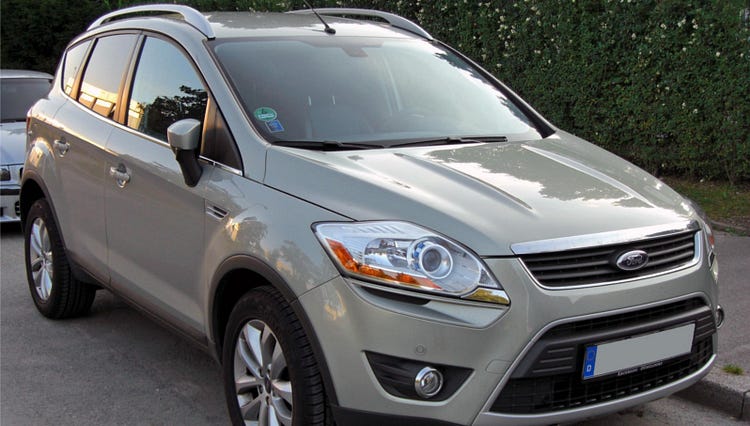
If you use it in the right way, then yes! What is the right way you ask? Well, sometimes not all augmentation techniques make sense for a dataset. Consider our car example again. Below are some of the ways by which you can modify the image.

Sure, they are pictures of the same car, but your target application may never see cars presented in these orientations.
For instance, if you’re just going to classify random cars on the road, only the second image would make sense to be on the dataset. But, if you own an insurance company that deals with car accidents, and you want to identify models of upside-down, broken cars as well, the third image makes sense. The last image may not make sense for both the above scenarios.
The point is, while using augmentation techniques, we have to make sure to not increase irrelevant data.
Is it really worth the effort?
You’re probably expecting some results to motivate you to walk the extra mile. Fair enough; I’ve got that covered too. Let me prove that augmentation really works, using a toy example. You can replicate this experiment to verify.
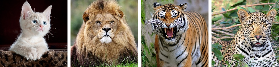
Let’s create two neural networks to classify data to one among four classes: cat, lion, tiger or a leopard. The catch is, one will not use data augmentation, whereas the other will. You can download the dataset from here link.
If you’ve checked out the dataset, you’ll notice that there’s only 50 images per class for both training and testing. Clearly, we can’t use augmentation for one of the classifiers. To make the odds more fair, we use Transfer Learning to give the models a better chance with the scarce amount of data.
For the one without augmentation, let’s use a VGG19 network. I’ve written a TensorFlow implementation here, which is based on this implementation. Once you’ve cloned my repo, you can get the dataset from here, and vgg19.npy (used for transfer learning) from here. You can now run the model to verify the performance.
I would agree though, writing extra code for data augmentation is indeed a bit of an effort. So, to build our second model, I turned to Nanonets. They internally use transfer learning and data augmentation to provide the best results using minimal data. All you need to do is upload the data on their website, and wait until it’s trained in their servers (Usually around 30 minutes). What do you know, it’s perfect for our comparison experiment.
Once it’s done training, you can request calls to their API to calculate the test accuracy. Checkout out my repo for a sample code snippet(Don’t forget to insert your model’s ID in the code snippet).
Results
VGG19 (No Augmentation)- 76% Test Accuracy (Highest)
Nanonets (With Augmentation) - 94.5% Test Accuracy
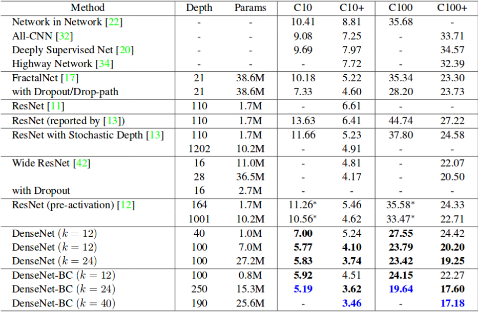
Impressive isn’t it. It is a fact that most models perform well with more data. So to provide a concrete proof, I’ve mentioned the table below. It shows the error rate of popular neural networks on the Cifar 10 (C10) and Cifar 100 (C100) datasets. C10+ and C100+ columns are the error rates with data augmentation.
Thank you for reading this article! Hope it shed some light about data augmentation. If you have any questions, you could hit me up on social media or send me an email (bharathrajn98@gmail.com).
This post was originally published on Nanonets. Reposted with permission.
About Nanonets: Nanonets is building APIs to simplify deep learning for developers. Visit them at https://www.nanonets.com for more
Related: