Data Augmentation For Bounding Boxes: Rethinking image transforms for object detection

comments

Random Horizontal Flip

 
First, we import all the necessary stuff and make sure the path is added even if we call the functions from outside the folder containing the files.  The following code goes in the file data_aug.py

import random
import numpy as np
import cv2
import matplotlib.pyplot as plt
import sys
import os

lib_path = os.path.join(os.path.realpath("."), "data_aug")
sys.path.append(lib_path)

The data augmentation will be implementing is RandomHorizontalFlip which flips an image horizontally with a probability p.

We first start by defining the class, and it's __init__ method. The init method contains the parameters of the augmentation. For this augmentation it is the probability with each image is flipped. For another augmentation like rotation, it may contain the  angle by which the object is to be rotated.

class RandomHorizontalFlip(object):
    
    """Randomly horizontally flips the Image with the probability *p*
    
    Parameters
    ----------
    p: float
        The probability with which the image is flipped
        
        
    Returns
    -------
    
    numpy.ndaaray
        Flipped image in the numpy format of shape `HxWxC`
    
    numpy.ndarray
        Tranformed bounding box co-ordinates of the format `n x 4` where n is 
        number of bounding boxes and 4 represents `x1,y1,x2,y2` of the box
        
    """

    def __init__(self, p=0.5):
        self.p = p

The docstring of the function has been written in Numpy docstring format. This will be useful to generate documentation using Sphinx.

The __init__ method of each function is used to define all the parameters of the augmentation. However, the actually logic of the augmentation is defined in the   __call__ function.

The call function, when invoked from a class instance takes two arguments, img and bboxeswhere img is the OpenCV numpy array containing the pixel values and bboxes is the numpy array containing the bounding box annotations.

The __call__ function also returns the same arguments, and this helps us chain together a bunch of augmentations to be applied in a Sequence.

def __call__(self, img, bboxes):
        img_center = np.array(img.shape[:2])[::-1]/2
        img_center = np.hstack((img_center, img_center))
        if random.random() < self.p:
            img =  img[:,::-1,:]
            bboxes[:,[0,2]] += 2*(img_center[[0,2]] - bboxes[:,[0,2]])
            
            box_w = abs(bboxes[:,0] - bboxes[:,2])
             
            bboxes[:,0] -= box_w
            bboxes[:,2] += box_w
            
        return img, bboxes

Let us break by bit by bit what's going on in here.

In a horizontal flip, we rotate the image about a verticle line passing through its center.

The new coordinates of each corner can be then described as the mirror image of the corner in the vertical line passing through the center of the image. For the mathematically inclined, the vertical line passing through the center would be the perpendicular bisector of the line joining the original corner and the new, transformed corner.

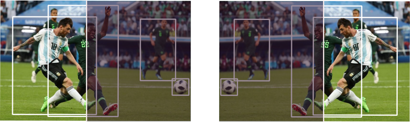
To have a better understanding of what is going on, consider the following image. The pixels in the right half of the transformed image and the left half of the original image are mirror images of each other about the central line.

The above is accomplished by the following piece of code.

img_center = np.array(img.shape[:2])[::-1]/2
img_center = np.hstack((img_center, img_center))
if random.random() < self.p:
   img =  img[:,::-1,:]
   bboxes[:,[0,2]] += 2*(img_center[[0,2]] - bboxes[:,[0,2]])

Note that the line img = img[:,::-1,:] basically takes the array containing the image and reverses it's elements in the 1st dimension, or the dimensional which stores the x-coordinates of the pixel values.

However, one must notice that the mirror image of the top left corner is the top right corner of the resultant box. Infact, the resultant coordinates are the top-right as well as bottom-left coordinates of the bounding box. However, we need them in the top-left and bottom right format.

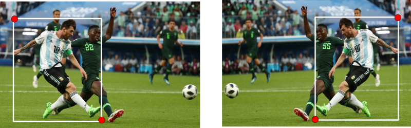
The side-effect of our code

The following piece of code takes care of the conversion.

box_w = abs(bboxes[:,0] - bboxes[:,2])
bboxes[:,0] -= box_w
bboxes[:,2] += box_w

We end up by returning the image and the array containing the bounding boxes.

Deterministic Version of HorizontalFlip

 
The above code applies the transformation stochastically with the probability p. However, if we want to build a deterministic version we can simply pass the argument p as 1. Or we could write another class, where we do not have the parameter p at all, and implement the __call__function like this.

def __call__(self, img, bboxes):
        img_center = np.array(img.shape[:2])[::-1]/2
        img_center = np.hstack((img_center, img_center))
        
        img =  img[:,::-1,:]
        bboxes[:,[0,2]] += 2*(img_center[[0,2]] - bboxes[:,[0,2]])
        
        box_w = abs(bboxes[:,0] - bboxes[:,2])
         
        bboxes[:,0] -= box_w
        bboxes[:,2] += box_w
        
    return img, bboxes

Seeing it in action

 
Now, let's suppose you have to use the HorizontalFlip augmentation with your images. We will use it on one image, but you can use it on any number you like. First, we create a file test.py. We begin by importing all the good stuff.

from data_aug.data_aug import *
import cv2 
import pickle as pkl
import numpy as np 
import matplotlib.pyplot as plt

Then, we import the image and load the annotation.

img = cv2.imread("messi.jpg")[:,:,::-1] #OpenCV uses BGR channels
bboxes = pkl.load(open("messi_ann.pkl", "rb"))

#print(bboxes)   #visual inspection

In order to see whether our augmentation really worked or not, we define a helper function draw_rect which takes in img and bboxes and returns a numpy image array, with the bounding boxes drawn on that image.

Let us create a file bbox_utils.py and import the neccasary stuff.

import cv2 
import numpy as np

Now, we define the function draw_rect

def draw_rect(im, cords, color = None):
    """Draw the rectangle on the image
    
    Parameters
    ----------
    
    im : numpy.ndarray
        numpy image 
    
    cords: numpy.ndarray
        Numpy array containing bounding boxes of shape `N X 4` where N is the 
        number of bounding boxes and the bounding boxes are represented in the
        format `x1 y1 x2 y2`
        
    Returns
    -------
    
    numpy.ndarray
        numpy image with bounding boxes drawn on it
        
    """
    
    im = im.copy()
    
    cords = cords.reshape(-1,4)
    if not color:
        color = [255,255,255]
    for cord in cords:
        
        pt1, pt2 = (cord[0], cord[1]) , (cord[2], cord[3])
                
        pt1 = int(pt1[0]), int(pt1[1])
        pt2 = int(pt2[0]), int(pt2[1])
    
        im = cv2.rectangle(im.copy(), pt1, pt2, color, int(max(im.shape[:2])/200))
    return im

Once, this is done, let us go back to our test.py file, and plot the original bounding boxes.

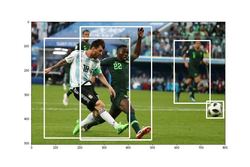
plt.imshow(draw_rect(img, bboxes))

This produces something like this.

Let us see the effect of our transformation.

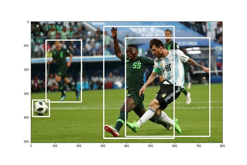
hor_flip = RandomHorizontalFlip(1)  

img, bboxes = hor_flip(img, bboxes)

plt.imshow(draw_rect(img, bboxes))

You should get something like this:

Takeaway Lessons

• The bounding box annotation should be stored in a numpy array of size N x 5, where N is the number of objects, and each box is represented by a row having 5 attributes; the coordinates of the top-left corner, the coordinates of the bottom right corner and the class of the object.
• Each data augmentation is defined as a class, where the __init__ method is used to define the parameters of the augmentation whereas the __call__ method describes the actual logic of the augmentation. It takes two arguments, the image img and the bounding box annotations bboxes and returns the transformed values.

This is it for this article. In the next article we will be dealing with Scale and Translateaugmentations. Not only they are more complex transformations, given there are more parameters (the scaling and translation factors), but also bring some challenges that we didn't have to deal with in the HorizontalFlip transformation. An example is to decide whether to retain a box if a portion of it is outside the image after the augmentation.

 
Bio: Ayoosh Kathuria currently an intern at the Defense Research and Development Organization, India, where he is working on improving object detection in grainy videos. When he's not working, he's either sleeping or playing pink floyd on his guitar. You can connect with him on LinkedIn or look at more of what he does at GitHub.

Original. Reposted with permission.

Related:

• How to Implement a YOLO (v3) Object Detector from Scratch in PyTorch: Part 1
• Building a Toy Detector with Tensorflow Object Detection API
• Getting Started with PyTorch Part 1: Understanding How Automatic Differentiation Works