Explainable Artificial Intelligence (Part 2) – Model Interpretation Strategies

The Accuracy vs. Interpretability Trade-off

 
There exists a typical Trade-off between Model Performance and Interpretability just like we have our standard Bias vs. Variance Trade-off in machine learning. In the industry, you will often hear that business stakeholders tend to prefer models which are more interpretable like linear models (linear\logistic regression) and trees which are intuitive, easy to validate and explain to a non-expert in data science. This increases the trust of people in these models since its decision policies are easier to understand. However, if you talk to data scientists solving real-world problems in the industry, they will tell you that due to the inherent high-dimensional and complex nature of real-world datasets, they often have to leverage machine learning models which might be non-linear and more complex in nature which are often impossible to explain using traditional methods (ensembles, neural networks). Thus, data scientists spend a lot of their time trying to improve model performance but in the process trying to strike a balance between model performance and interpretability.

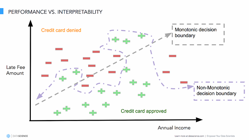
Model performance vs. interpretability (Source: https://www.datascience.com)

The above figure shows us model decision boundaries for a customer loan approval problem. We can clearly see that simple, easy to interpret models with monotonic decision boundaries may work fine in certain scenarios but usually in real-world scenarios and datasets, we end up using a more complex and hard to interpret model having a non-monotonic decision boundary. Hence to reinforce our motivation, we need model interpretation such that, we are able to account for fairness (unbiasedness/non-discriminative), accountability (reliable results) and transparency (being able to query and validate predictive decisions) of a predictive model. Interested readers should check out the article, “Toward the Jet Age of machine learning”. Besides this, I would definitely recommend readers to check out my personal favorite, and an article from which I adapted a lot of content in this series, “Interpreting predictive models with Skater: Unboxing model opacity” which talks about this in further detail.

Interpreting predictive models with Skater: Unboxing model opacity
A deep dive into model interpretation as a theoretical concept and a high-level overview of Skater.www.oreilly.com

 

Model Interpretation Techniques

 
There are a wide variety of new model interpretation techniques which try to address the limitations and challenges of traditional model interpretation techniques and try to combat the classic Intepretability vs. Model Performance Trade-off. In this section, we will take a look at some of these techniques and strategies. Remember, our focus will be to cover model-agnostic interpretation techniques since these techniques are truly going to help us on the road in our journey towards Explainable AI (XAI).

 
Using Interpretable Models
The easiest way to get started with model interpretation is to use models which are interpretable out of the box! This typically includes your regular parametric models like linear regression, logistic regression, tree-based models, rule-fits and even models like k-nearest neighbors and Naive Bayes! A way to categorize these models based on their major capabilities would be:

• Linearity: Typically we have a linear model model if the association between features and target is modeled linearly.
• Monotonicity: A monotonic model ensures that the relationship between a feature and the target outcome is always in one consistent direction (increase or decrease) over the feature (in its entirety of its range of values).
• Interactions: You can always add interaction features, non-linearity to a model with manual feature engineering. Some models create it automatically also.

Christoph Molnar’s excellent book, ‘Interpretable Machine Learning’ has a nice table summarizing the above aspects.

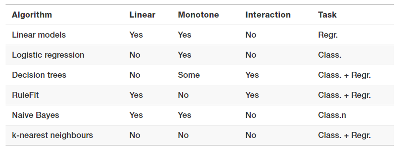
Source: Interpretable Machine Learning, Christoph Molnar

A good point to remember is that some of these models might be too simplistic and hence we might need to think of better ways to build and interpret more complex and better performing models.

 
Feature Importance

Feature importance is generic term for the degree to which a predictive model relies on a particular feature. Typically, a feature’s importance is the increase in the model’s prediction error after we permuted the feature’s values. Frameworks like Skater compute this based on an information theoretic criteria, measuring the entropy in the change of predictions, given a perturbation of a given feature. The intuition is that the more a model’s decision criteria depend on a feature, the more we’ll see predictions change as a function of perturbing a feature. However, frameworks like SHAP, use a combination of feature contributions and game theory to come up with SHAP values. Then, it computes the global feature importance by taking the average of the SHAP value magnitudes across the dataset. Following is a standard example of a feature importance plot from Skater on a census dataset.

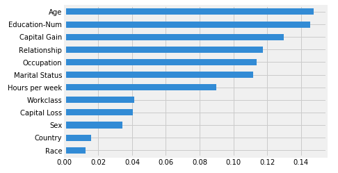
Looks like Age and Education-Num are the top two features, where Age is reponsible for model predictions changing by an average of 14.5% on perturbing\permuting the Age feature. Hence, to summarize, the concept behind global interpretations of model-agnostic feature importance is really straightforward.

• We measure a feature’s importance by calculating the increase of the model’s prediction error after perturbing the feature.
• A feature is “important” if perturbing its values increases the model error, because the model relied on the feature for the prediction.
• A feature is “unimportant” if perturbing its values keeps the model error unchanged, because the model basically ignored the feature for the prediction.

The permutation feature importance measurement was introduced for Random Forests by Breiman (2001). Based on this idea, Fisher, Rudin, and Dominici (2018) proposed a model-agnostic version of the feature importance — they called it Model Reliance.

 
Partial Dependence Plots

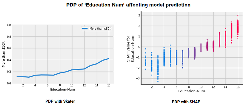
Partial Dependence describes the marginal impact of a feature on model prediction, holding other features in the model constant. The derivative of partial dependence describes the impact of a feature (analogous to a feature coefficient in a regression model). The partial dependence plot (PDP or PD plot) shows the marginal effect of a feature on the predicted outcome of a previously fit model. PDPs can show if the relationship between the target and a feature is linear, monotonic or more complex. The partial dependence plot is a global method: The method takes into account all instances and makes a statement about the global relationship of a feature with the predicted outcome. Following figures show some example PDPs.

PDP for 1 feature

We have leveraged Skater and SHAP to show the effect of Education Level on earning more money here. This is a one-way PDP showing the effect of one feature on the model predictions. We can also build two-way PDPs showing the effect of two features on model predictions. An example is illustrated in the following figure.

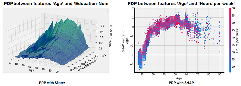
PDP for 2 features

You can clearly see the effect and interaction of the features which influence the model predictions in the above PDPs. Notable middle-aged people with higher education levels and more working hours per week earn more money!

 
Global Surrogate Models

We have see various ways to interpret machine learning models with feature importances, dependence plots, less complex models. But is there a way to build intepretable approximations of really complex models? Thankfully we have global surrogate models just for this purpose! A global surrogate model is an interpretable model that is trained to approximate the predictions of a black box model which can essentially be any model regardless of its complexity or training algorithm — this is as model-agnostic as it gets!

Typically we approximate a more interpretable surrogate model based on our base model which is treated as a black box model. We can then draw conclusions about the black box model by interpreting the surrogate model. Solving machine learning interpretability by using more machine learning!

The purpose of (interpretable) surrogate models is to approximate the predictions of the underlying model as closely as possible while being interpretable. Fitting a surrogate model is a model-agnostic method, since it requires no information about the inner workings of the black box model, only the relation of input and predicted output is used. The choice of the base black box model type and of the surrogate model type is decoupled. Tree-based models are not too simplistic but interpretable and make a good choice for building surrogate models.

Skater introduce the novel idea of using TreeSurrogates as means for explaining a model's learned decision policies (for inductive learning tasks), which is inspired by the work of Mark W. Craven described as the TREPAN algorithm. We will be covering the TREPAN model with examples in Part 3 of this series. For now, Christoph Molnar, does an excellent job in talking about the main steps involved for building surrogate models in his book.

1. Choose a dataset This could be the same dataset that was used for training the black box model or a new dataset from the same distribution. You could even choose a subset of the data or a grid of points, depending on your application.
2. For the chosen dataset, get the predictions of your base black box model.
3. Choose an interpretable surrogate model (linear model, decision tree, …).
4. Train the interpretable model on the dataset and its predictions.
5. Congratulations! You now have a surrogate model.
6. Measure how well the surrogate model replicates the prediction of the black box model.
7. Interpret / visualize the surrogate model.

Of course this is a high level illustration and algorithms like TREPAN do a lot more internally but the overall workflow still remains the same.

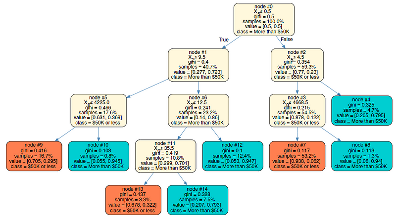
Sample illustration of a surrogate tree model

The above illustration is of a surrogate tree model approximated from a complex XGBoost black box model. We will be building this from scratch in Part 3 so stay tuned! Interestingly this model has an overall accuracy of 83% as compared to the XGBoost model’s accuracy which is 87%. Not bad!

 
Local Interpretable Model-agnostic Explanations (LIME)

LIME is a novel algorithm designed by Riberio Marco, Singh Sameer, Guestrin Carlos to access the behavior of the any base estimator(model) using local interpretable surrogate models (e.g. linear classifier/regressor). Such form of comprehensive evaluation helps in generating explanations which are locally faithful but may not align with the global behavior. Basically, LIME explanations are based on local surrogate models. These, surrogate models are interpretable models (like a linear model or decision tree) that are learned on the predictions of the original black box model. But instead of trying to fit a global surrogate model, LIME focuses on fitting local surrogate models to explain why single predictions were made. In fact, LIME is also available as an open-source framework on GitHub and is based on the work presented in this paper.

The idea is very intuitive. To start with, just try and unlearn what you have done so far! Forget about the training data, forget about how your model works! Think that your model is a black box model with some magic happening inside, where you can input data points and get the models predicted outcomes. You can probe this magic black box as often as you want with inputs and get output predictions. Now, you main objective is to understand why the machine learning model which you are treating as a magic black box, gave the outcome it produced. LIME tries to do this for you! It tests out what happens to you black box model’s predictions when you feed variations or perturbations of your dataset into the black box model. Typically, LIME generates a new dataset consisting of perturbed samples and the associated black box model’s predictions. On this dataset LIME then trains an interpretable model weighted by the proximity of the sampled instances to the instance of interest. Following is a standard high-level workflow for this.

• Choose your instance of interest for which you want to have an explanation of the predictions of your black box model.
• Perturb your dataset and get the black box predictions for these new points.
• Weight the new samples by their proximity to the instance of interest.
• Fit a weighted, interpretable (surrogate) model on the dataset with the variations.
• Explain prediction by interpreting the local model.

Following is a sample example of LIME in action in the Skater framework explaining why the model predicted a person will earn more than $50K.

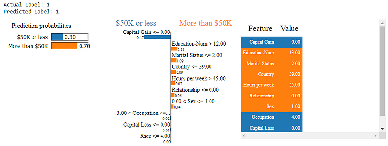
Explaining predictions with LIME

We will be using the Census dataset to build models and explore them with LIME in our next article in further detail.

 
Shapley Values and SHapley Additive exPlanations (SHAP)

SHAP (SHapley Additive exPlanations) is a unified approach to explain the output of any machine learning model. SHAP connects game theory with local explanations, uniting several previous methods and representing the only possible consistent and locally accurate additive feature attribution method based on what they claim! (do check out the SHAP NIPS paper for details). SHAP is an excellent model interpretation framework which is based on adaptation and enhancements to Shapley values which we shall explore in-depth in this section. Thanks once again to Christoph Molnar’s amazing model interpretation book which I shall be shamelessly adapting into this tutorial because in my opinion that is perhaps the best way to understand this concept!

Typically, model predictions can be explained by assuming that each feature is a ‘player’ in a game where the prediction is the payout. The Shapley value — a method from coalitional game theory — tells us how to fairly distribute the ‘payout’ among the features. Let’s take an illustrative example.

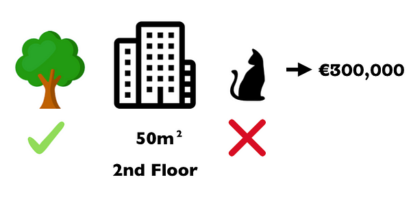
Assume you trained a machine learning model to predict apartment prices. For a certain apartment it predicts 300,000 € and you need to explain this prediction. The apartment has a size of 50 m-sq, is located on the 2nd floor, with a park nearbyand cats are forbidden. The average prediction for all apartments is 310,000€. How much did each feature value contribute to the prediction compared to the average prediction?

The answer is easy for linear regression models: The effect of each feature is the weight of the feature times the feature value minus the average effect of all apartments: This works only because of the linearity of the model. For more complex models what do we do? One option is LIME which we just discussed. A different solution comes from cooperative game theory: The Shapley value, coined by Shapley, is a method for assigning payouts to players depending on their contribution towards the total payout. Players cooperate in a coalition and obtain a certain gain from that cooperation.

• The ‘game’ is the prediction task for a single instance of the dataset.
• The ‘gain’ is the actual prediction for this instance minus the average prediction of all instances.
• The ‘players’ are the feature values of the instance, which collaborate to receive the gain (= predict a certain value).

Thus, in our apartment example, the feature values ‘park-allowed’, ‘cat-forbidden’, ‘area-50m-sq’ and ‘floor-2nd’ worked together to achieve the prediction of 300,000€. Our goal is to explain the difference of the actual prediction (300,000€) and the average prediction (310,000€): a difference of -10,000€. The answer could be: The ‘park-nearby’ contributed 30,000€; ‘size-50m-sq’ contributed 10,000€; ‘floor-2nd’ contributed 0€; ‘cat-forbidden’ contributed -50,000€. The contributions add up to -10,000€: the final prediction minus the average predicted apartment price.
The Shapley value is the average marginal contribution of a feature value over all possible coalitions. Coalitions are basically combinations of features which are used to estimate the shapley value of a specific feature. Typically more the features, it starts increasing exponentially hence it may take a lot of time to compute these values for big or wide datasets. The following figure shows all coalitions of feature values that are needed to assess the Shapley value for ‘cat-forbidden’.

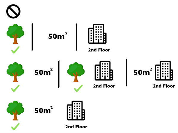
The first row shows the coalition without any feature values. The 2nd, 3rd and 4th row show different coalitions — separated by ‘|’ — with increasing coalition size. For each of those coalitions we compute the predicted apartment price with and without the ‘cat-forbidden’ feature value and take the difference to get the marginal contribution. The Shapley value is the (weighted) average of marginal contributions. We replace the feature values of features that are not in a coalition with random feature values from the apartment dataset to get a prediction from the machine learning model. When we repeat the Shapley value for all feature values, we get the complete distribution of the prediction (minus the average) among the feature values. SHAP is an enhancement on the Shapley values.

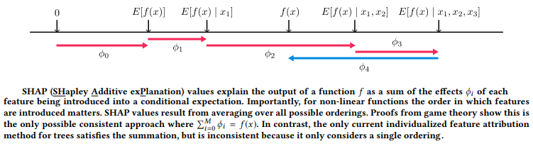
SHAP (SHapley Additive exPlanations) assigns each feature an importance value for a particular prediction. Its novel components include: the identification of a new class of additive feature importance measures, and theoretical results showing there is a unique solution in this class with a set of desirable properties. Typically, SHAP values try to explain the output of a model (function) as a sum of the effects of each feature being introduced into a conditional expectation. Importantly, for non-linear functions the order in which features are introduced matters. The SHAP values result from averaging over all possible orderings. Proofs from game theory show this is the only possible consistent approach. The following figure from the KDD 18 paper, Consistent Individualized Feature Attribution for Tree Ensemblessummarizes this in a nice way!

Understanding SHAP value

Following is an illustration of using SHAP to explaining the model’s decisions when it’s predicting if a person’s income > $50K

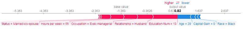
Explaining model predictions with SHAP

It is interesting to see the key drivers (features) behind the model taking such a decision! We will also be covering this with hands-on examples in Part 3 of this series.

 

Conclusion

 
This article should help you take more definitive steps on the road towards Explanable AI (XAI). You now know the need and importance of model interpretation. The issues with bias and fairness from the first article. Here we have taken a look at traditional techniques for model interpretation, discussed their challenges and limitations and also covered the classic trade-off between model interpretability and prediction performance. Finally, we looked at the current state-of-the-art model interpretation techniques and strategies including feature importances, PDPs, global surrogates, local surrogates and LIME, shapley values and SHAP. Like I have mentioned before, Let’s try and work towards human-interpretable machine learning and XAI to demystify machine learning for everyone and help increase the trust in model decisions.

 

What’s next?

 
In Part 3 of this series, we will be looking at a comprehensive guide to building and interpreting machine learning models using all the new techniques we learnt in this article. We will be using several state-of-the-art model interpretation frameworks for this.

• Hands-on guides on using the latest state-of-the-art model interpretation frameworks
• Features, concepts and examples of using frameworks like ELI5, Skater and SHAP
• Explore concepts and see them in action — Feature importances, partial dependence plots, surrogate models, interpretation and explanations with LIME, SHAP values
• Hands-on Machine Learning Model Interpretation on a supervised learning example

Stay tuned, this is definitely going to get more interesting and exciting!

 
Check out ‘Part I — The Importance of Human Interpretable Machine Learning’ which covers the what and why of human interpretable machine learning and the need and importance of model interpretation along with its scope and criteria in case you haven’t!
Thanks to all the wonderful folks at DataScience.com and especially Pramit Choudhary for building an amazing model interpretation framework, Skater,and helping me out with some excellent content for this series.

I cover a lot of examples of machine learning model interpretation in my book, “Practical Machine Learning with Python”. The code is open-sourced for your benefit!

Have feedback for me? Or interested in working with me on research, data science, artificial intelligence or even publishing an article on TDS? You can reach out to me on LinkedIn.

 
Bio: Dipanjan Sarkar is a Data Scientist @Intel, an author, a mentor @Springboard, a writer, and a sports and sitcom addict.

Original. Reposted with permission.

Related:

• Human Interpretable Machine Learning (Part 1) — The Need and Importance of Model Interpretation
• Emotion and Sentiment Analysis: A Practitioner’s Guide to NLP
• Named Entity Recognition: A Practitioner’s Guide to NLP