Boost Your Image Classification Model

By Aditya Mishra, ML Engineer at difference-engine.ai

Image classification is assumed to be a nearly solved problem. Fun part is when you have to use all your cunning to gain that extra 1% accuracy. I came across such a situation, when I participated in Intel Scene Classification Challenge hosted by Analytics Vidhya. I thoroughly enjoyed the contest as I tried to extract out all the juices from my deep learning model. The techniques below can in general be applied to any image classification problem at hand.

 

Problem

 
The problem was to classify a given image into 6 categories

 

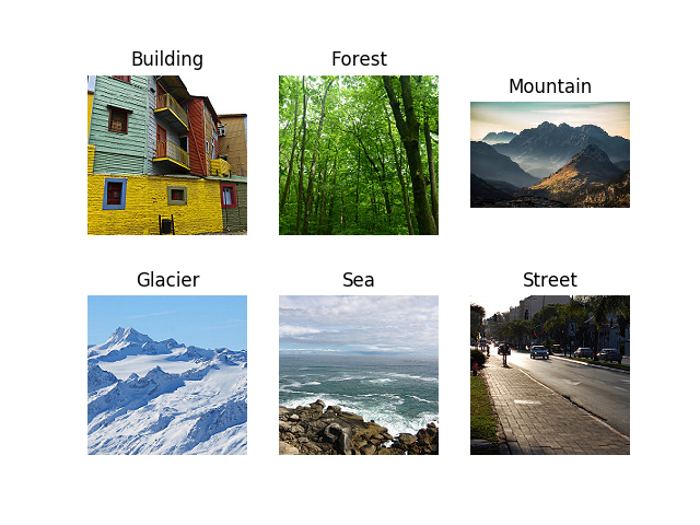
We were given ~25K images from a wide range of natural scenes from all around the world

 

Progressive Resizing

 
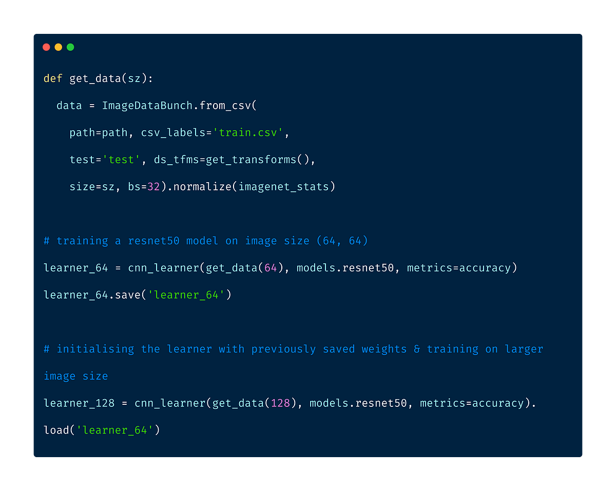
It is the technique to sequentially resize all the images while training the CNNs on smaller to bigger image sizes. Progressive Resizing is described briefly in his terrific fastai course, “Practical Deep Learning for Coders”. A great way to use this technique is to train a model with smaller image size say 64x64, then use the weights of this model to train another model on images of size 128x128 and so on. Each larger-scale model incorporates the previous smaller-scale model layers and weights in its architecture.

 

 

FastAI

 

The fastai library is a powerful deep learning library. If the FastAI team finds a particularly interesting paper, they test it out on different datasets & work out how to tune it. Once successful, it gets incorporated in their library, and is readily available for its users. The library contains many State of the art (SOTA)techniques built in. Built on type of pytorch, fastai has excellent default parameters for most if not all the tasks. Some of the techniques are

1. Cyclical Learning Rate
2. One cycle learning
3. Deep Learning on Structured Data

 

Sane weight initialization

 
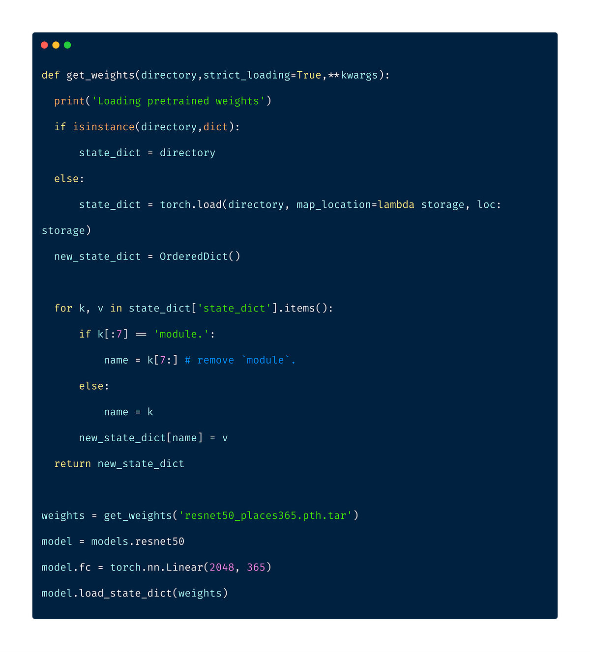
While checking out standard datasets available, I stumbled across Places365 dataset. The Places365 dataset contains 1.8 million images from 365 scene categories. The dataset provided in the challenge was very similar to this dataset, so the model trained on this dataset will already have learned features that are relevant to our own classification problem. As, the categories in our problem, was a subset of Places365 dataset, I used a ResNet50 model initialised with places365 weights.

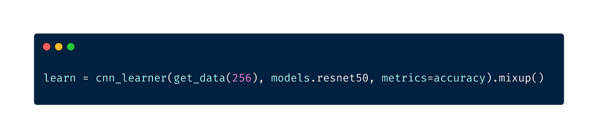
The model weights were available as pytorch weights. The below utility function helped us load the data properly into fastai’s CNN Learner.

 

Mixup Augmentation

 
Mixup augmentation is a type of augmentation where in we form a new image through weighted linear interpolation of two existing images. We take two images and do a linear combination of them in terms of tensors of those images.

 

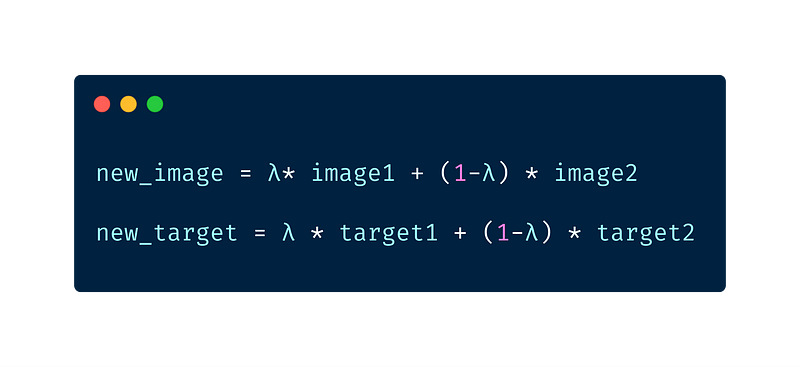
λ is randomly sampled from the beta distribution. Even though the authors of the paper suggest using λ=0.4, the default value in the fastai library is set to 0.1

 

 

Learning Rate Tuning

 
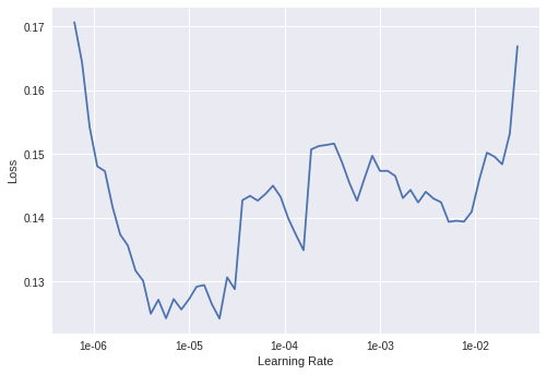
Learning rate is one of the most important hyper-parameter for training neural networks. fastai has a method to find out an appropriate initial learning rate. This technique is called cyclical learning rate, wherein we run a trial with a lower learning rate & increase it exponentially, recording the loss along the way. We then plot the loss against learning rate & choose the learning rate where the loss is the steepest.

 

 

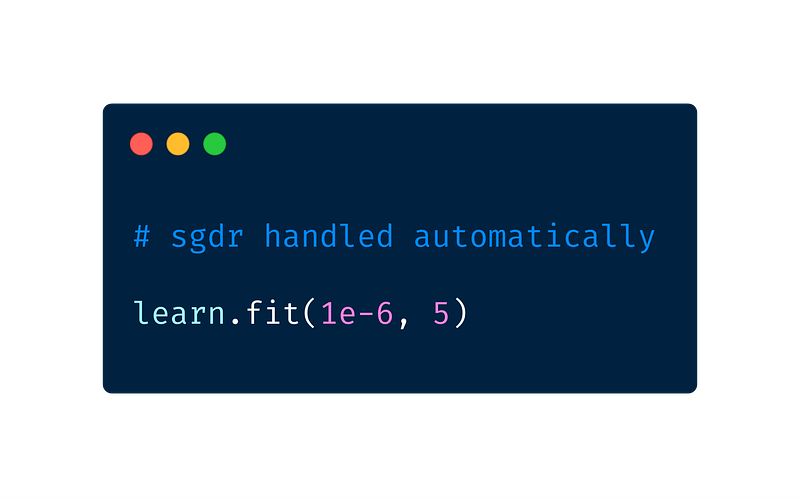
The library also handles Stochastic Gradient Descent with Restart (SGDR) for us automatically. In SGDR, the learning rate is reset at the start of each epoch to the original chosen value which decreases over the epoch as in Cosine Annealing. The main benefit of this, is that since the learning rate is reset at start of each epoch, the learner is capable of jumping out of a local minima or a saddle point it may be stuck in.

 

 

General Adversarial Networks

 
GANs were introduced by Ian Goodfellow in 2014. GANs are deep neural net architectures comprised of two nets, pitting one against the other. GANs can mimic any distribution of data. They can learn to generate data similar to the original data in any domain-images, speech, text, etc. We used fast.ai’s Wasserstein GAN implementation to generate more training images.

GANs involve training two neural networks, one called the generator, which generates new data instances, while the other, the discriminator, evaluates them for authenticity, it decides whether each instance of data belongs to the actual training dataset or not. You can refer more about it here.

 

 

Removing Confusing Images

 

The first step to training a neural net is to not touch any neural net code at all and instead begin by thoroughly inspecting your data. This step is critical. I like to spend copious amount of time (measured in units of hours) scanning through thousands of examples, understanding their distribution and looking for patterns.

- Andrej Karpathy

As Andrej Karpathy states “Data Investigation” is an important step. Upon data investigation, I found that there were some images which contained 2 or more classes.

Approach 1

Using a previously trained model, I ran prediction on the entire training data. Then discarded those images whose predictions were incorrect but the probability score was more than 0.9. These were the images, that the model clearly misclassified. Going deep into it, I found that those images were mislabelled by the labeller.

 

I also removed those images from the training set, for whom the prediction probability was in the range 0.5 to 0.6, the theory being that there might be more than 1 class present in the image, so the model assigned somewhat equal probabilities to each one of them. Upon viewing those images, the theory turned out to be true in the end

Approach 2

fast.ai provides a handy widget “Image Cleaner Widget” that allows you to clean and prepare your data for your model. ImageCleaner is for cleaning up images that don’t belong in your dataset. It renders images in a row and gives you the opportunity to delete the file from your file system.

 

Test Time Augmentation

 
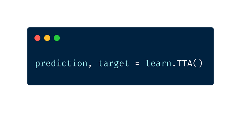
Test Time Augmentation involves taking a series of different versions of the original image and passing them through the model. The average output is then calculated from the different versions and given as the final output for the image.

 

A similar technique called 10-crop testing was used previously. I first read about 10-crop technique in ResNet paper. The 10-crop technique involves cropping the original image along the four corners and once along the centre giving 5 images. Repeating the same for the it’s inverse, gives another 5 images, a total of 10 images. Test time augmentation is however faster then 10-crop technique

 

Ensembling

 
Ensembling in machine learning is the technique of using multiple learning algorithms to obtain better predictive performance then that could be achieved by a single algorithm. Ensembling works best

1. Constituent models are of different natures. Eg, ensembling a ResNet50 and InceptionNet would be much more useful then combining a ResNet50 and ResNet34 net as they are different in nature
2. Constituent models have lower correlation
3. Changing training set for each of the models; so that there is more variation

In this case, I ensembled the prediction from all the models by picking the maximum occuring class. In case there’s more than one class having maximum occurence, I randomly pick one of the classes.

 

Results

 

Public Leaderboard — Rank 29 (0.962)

Private Leaderboard — Rank 22 (0.9499)

 

Conclusion

 

1. Progressive resizing is a great idea to get started.
2. Spending time understanding your data & visualising it is must.
3. A great deep learning library like fastai with sensibly initialised parameters definitely helps.
4. Use transfer learning wherever & whenever possible, as it usually gives good results. Recently, deep learning & transfer learning has even been applied to structured data, so transfer learning should definitely be the first thing to try out.
5. State of the art techniques like Mixup Augmentation, TTA, Cyclic LR would definitely help you push your accuracy score by those extra 1 or 2%.
6. Always search for datasets that are relevant to your problem & use include them in your training data if possible. If there exists, deep learning models trained on these datasets, use their weights as initial weights for your model.

 
Bio: Aditya Mishra is an ML Engineer at difference-engine.ai.

Original. Reposted with permission.

Related:

• Large-Scale Evolution of Image Classifiers
• Building NLP Classifiers Cheaply With Transfer Learning and Weak Supervision
• How to do Everything in Computer Vision