From Data Pre-processing to Optimizing a Regression Model Performance
All you need to know about data pre-processing, and how to build and optimize a regression model using Backward Elimination method in Python.

Coming up with features is difficult, time-consuming, requires expert knowledge. “Applied machine learning” is basically feature engineering.
— Andrew Ng, Stanford University(source)
Introduction
Machine learning (ML) helps in finding complex and potentially useful patterns in data. These patterns are fed to a Machine Learning model that can then be used on new data points — a process called making predictions or performing inference.
Building a Machine Learning model is a multistep process. Each step presents its own technical and conceptual challenges. In this article, we are going to focus on the process of selecting, transforming, and augmenting the source data to create powerful predictive signals to the target variable (in supervised learning). These operations combine domain knowledge with data science techniques. They are the essence of feature engineering.
This article explores the topic of data engineering and feature engineering for machine learning (ML). This first part discusses the best practices of preprocessing data in a regression model. The article focuses on using python’s pandas and sklearn library to prepare data, train the model, serve the model for prediction.
Table of Contents:
- Data pre-processing.
- Fitting Multiple Linear regression model
- Building an optimal Regression model using the backward elimination method
- Fine-tune the Regression model
Let us start with Data pre-processing…
1. What is Data pre-processing and why it is needed?
Data preprocessing is a data mining technique that involves transforming raw data into an understandable format. Real-world data is often incomplete: lacking attribute values, lacking certain attributes of interest, or containing only aggregate data, Noisy: containing errors or outliers. Inconsistent: containing discrepancies in codes or names. Data preprocessing is a proven method of resolving such issues.
In Real-world data are generally incomplete: lacking attribute values, lacking certain attributes of interest, or containing only aggregate data. Noisy: containing errors or outliers. Inconsistent: containing discrepancies in codes or names.
1.1) Steps in Data Preprocessing
Step 1: Import the libraries
Step 2: Import the data-set
Step 3: Check out the missing values
Step 4: Encode the Categorical data
Step 5: Splitting the dataset into Training and Test set
Step 6: Feature scaling
Let’s discuss all these steps in details.
Step 1: Import the libraries
A library is also a collection of implementations of behavior, written in terms of a language, that has a well-defined interface by which the behavior is invoked. For instance, people who want to write a higher-level program can use a library to make system calls instead of implementing those system calls over and over again. — Wikipedia
We need to import 3 essential python libraries.
1. Numpy is the fundamental package for scientific computing with Python.
2. Pandas is for data manipulation and analysis.
3. Matplotlib is a Python 2D plotting library which produces publication quality figures in a variety of hard copy formats and interactive environments across platforms.
import numpy
import matplotlib.pyplot as plt
import pandas as pd
Step 2: Import the data-set
Data is imported using the pandas library.
data = pd.read_csv('/path_of_your-dataset/Data.csv')
X = data.iloc[:,:-1].values
y = data.iloc[:,3].values
Here, X represents a matrix of independent variables and y represents a vector of the dependent variable.
Step 3: Check out the missing values
There are two ways by which we can handle missing values in our dataset. The first method commonly used to handle null values. Here, we either delete a particular row if it has a null value for a particular feature and a particular column if it has more than 75% of missing values. This method is advised only when there are enough samples in the data set. One has to make sure that after we have deleted the data, there is no addition of bias.
In the second method, we replace all the NaN values with either mean, median or most frequent value. This is an approximation which can add variance to the data set. But the loss of the data can be negated by this method which yields better results compared to removal of rows and columns. Replacing with the above three approximations are a statistical approach to handling the missing values. This method is also called as leaking the data while training.
For dealing with missing data, we will use Imputer library from sklearn.preprocessing package. Instead of providing mean you can also provide median or most frequent value in the strategy parameter.
from sklearn.preprocessing import Imputer
imputer = Imputer(missing_values='NaN', strategy = 'mean', axis = 0)
Next step is to train the imputer instance with the data stored in X(predictors).
imputer = imputer.fit(X[:,1:3])
X[:, 1:3] = imputer.transform(X[:,1:3])
Step 4: Encode the Categorical data
Categorical data are variables that contain label values rather than numeric values. The number of possible values is often limited to a fixed set.
Some examples include:
A “pet” variable with the values: “dog” and “cat”.
A “color” variable with the values: “red”, “green” and “blue”.
A “place” variable with the values: “first”, “second” and “third”.
Each value represents a different category.
Note: What is the Problem with Categorical Data?
Some algorithms can work with categorical data directly. But many machine learning algorithms cannot operate on label data directly. They require all input variables and output variables to be numeric.
In general, this is mostly a constraint of the efficient implementation of machine learning algorithms rather than hard limitations on the algorithms themselves. This means that categorical data must be converted to a numerical form. If the categorical variable is an output variable, you may also want to convert predictions by the model back into a categorical form in order to present them or use them in some application.
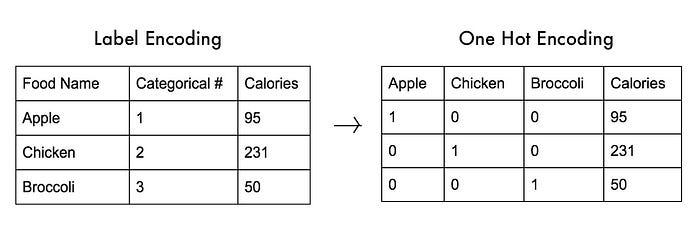
We are going to use a technique called label encoding. Label encoding is simply converting each value in a column to a number. For example, the body_style column contains 5 different values. We could choose to encode it like this:
- convertible -> 0
- hardtop -> 1
- hatchback -> 2
- sedan -> 3
- wagon -> 4
To implement Label encoding we will import LabelEncoder from sklearn.preprocessing package. But it labels categories as 0,1,2,3…. Now since 0<1<2, the equations in your regression model may thing one category has a higher value than the other, which is of course not true.
To solve this situation we have a concept called Dummy variables. In regression analysis, a dummy variable is one that takes the value 0 or 1 to indicate the absence or presence of some categorical effect that may be expected to shift the outcome. They are used as devices to sort data into mutually exclusive categories (such as smoker/non-smoker, etc.).
To implement the concept of dummy variables we will import OneHotEncoder library from sklearn.preprocessing package. You need to provide the column index which needs to be encoded under categorical_features. So if a column has 3 categories, 3 columns will be created and likewise for any number of categories.
from sklearn.preprocessing import LabelEncoder, OneHotEncoder
labelencoder_X = LabelEncoder()
X[:,0] = labelencoder_X.fit_transform(X[:,0])
onehotencoder = OneHotEncoder(categorical_features = [0])
X = onehotencoder.fit_transform(X).toarray()
Step 5: Splitting the dataset into Training and Test set
Second last step in our data pre-processing is splitting the data into training and test set.
from sklearn.model_selection import train_test_split
X_train, X_test, y_train, y_test =  train_test_split(X,y,test_size = 0.2, random_state= 0)
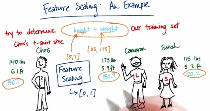
Step 6: Feature scaling
Feature scaling or data normalization is a method used to normalize the range of independent variables or features of data. So when the values vary a lot in an independent variable, we use feature scaling so that all the values remain in the comparable range.
6.1) Method of Feature scaling
- StandardScaler
- MinMaxScaler
- RobustScaler
- Normalizer
To implement feature scaling we need to import StandardScaler library from sklearn.preprocessing package. StandardScaler assumes your data is normally distributed within each feature and will scale them so that the distribution is now centered around 0, with a standard deviation of 1.
from sklearn.preprocessing import StandardScaler
sc_X = StandardScaler()
X_train = sc_X.fit_transform(X_train)
X_test = sc_X.transform(X_test)
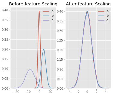
Demonstration of feature scaling graphically:
import pandas as pd
import numpy as np
from sklearn import preprocessing
import matplotlib
import matplotlib.pyplot as plt
import seaborn as sns
matplotlib.style.use('ggplot')
np.random.seed(1)
df = pd.DataFrame({
    'a': np.random.normal(0, 1, 5000),
    'b': np.random.normal(4, 2, 5000),
    'c': np.random.normal(-8, 4, 5000)
})

scaler = preprocessing.StandardScaler()
scaled_df = scaler.fit_transform(df)
scaled_df = pd.DataFrame(scaled_df, columns=['a', 'b', 'c'])
fig, (ax1, ax2) = plt.subplots(ncols=2, figsize=(6, 5))
ax1.set_title('Before feature Scaling')
sns.kdeplot(df['a'], ax=ax1)
sns.kdeplot(df['b'], ax=ax1)
sns.kdeplot(df['c'], ax=ax1)
ax2.set_title('After feature Scaling')
sns.kdeplot(scaled_df['a'], ax=ax2)
sns.kdeplot(scaled_df['b'], ax=ax2)
sns.kdeplot(scaled_df['c'], ax=ax2)
plt.show()
Here, a,b,c are three independent variables.
So finally we have our data pre-processing template ready and can be used in any regression analysis.
#Import essential libraries
import numpy
import matplotlib.pyplot as plt
import pandas as pd#Import the dataset
data = pd.read_csv('/path_of_your-dataset/Data.csv')
X = data.iloc[:,:-1].values
y = data.iloc[:,3].values #taking care of missing values
from sklearn.preprocessing import Imputer
imputer = Imputer(missing_values='NaN', strategy = 'mean', axis = 0)
imputer = imputer.fit(X[:,1:3])
X[:, 1:3] = imputer.transform(X[:,1:3]) #Encoding categorical data
from sklearn.preprocessing import LabelEncoder, OneHotEncoder
labelencoder_X = LabelEncoder()
X[:,0] = labelencoder_X.fit_transform(X[:,0])
onehotencoder = OneHotEncoder(categorical_features = [0])
X = onehotencoder.fit_transform(X).toarray() #encode target variable
labelencoder_y = LabelEncoder()
y = labelencoder_y.fit_transform(y) #splitting the dataset into test and training data
from sklearn.model_selection import train_test_split
X_train, X_test, y_train, y_test =  train_test_split(X,y,test_size = 0.2, random_state= 0)#feature scaling
from sklearn.preprocessing import StandardScaler
sc_X = StandardScaler()
X_train = sc_X.fit_transform(X_train)
X_test = sc_X.transform(X_test)
So we have our data pre-processing template completely ready and can be applied to any Regression analysis. Please note that all the steps discussed above are not compulsory for all the regression model because some models take care of most of the data preprocessing part.
In the next part, we are going to fit a Mulitple Linear Regression Model to the data.
2. Fitting a Multiple Linear Regression Model

You can download the dataset from here, contains 5 columns and 50 rows and it looks something like this:-
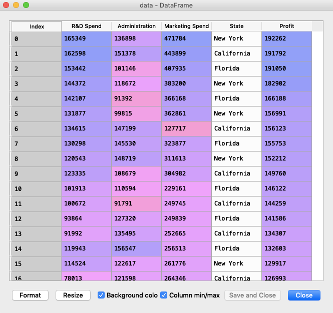
So our dataset contains columns R&D Spend, Administration, Marketing Spend, State and Profit. First four columns are our independent variables and Profit is our dependent/target variable.
Our goal is to train our regression model on 80% of the original data and then test it on the rest of the data.
Note — The dataset contains the state column which consists of categorical values. As we have already discussed that some regression models can work with text input but Multiple regression cannot, so we need to encode this column into numeric values using dummy variables(OneHotEncoder in sklearn).
Before moving ahead I think we should understand the Dummy Variable Trap.
Dummy Variable Trap: The phenomenon where one or several independent variables in a linear regression predict another and is called multicollinearity. As a result, the model cannot distinguish between the effects of one column on another column. So when you are building a model, always omit one dummy variable from the rest.
After performing all the steps of data pre-processing and building our multiple regression model our code looks something like this.
import numpy as np
import matplotlib.pyplot as plt
import pandas as pddata = pd.read_csv('/path_to_data/50_Startups.csv')
X = data.iloc[:,:-1].values
y = data.iloc[:,4].values #Encoding categorical data
from sklearn.preprocessing import LabelEncoder, OneHotEncoder
labelencoder_X = LabelEncoder()
X[:,3] = labelencoder_X.fit_transform(X[:,3])
onehotencoder = OneHotEncoder(categorical_features = [3])
X = onehotencoder.fit_transform(X).toarray() #avoiding dummy variable trap -> removing 1 column
X = X[:,1:] #splitting the dataset into test and training data
from sklearn.model_selection import train_test_split
X_train, X_test, y_train, y_test =  train_test_split(X,y,test_size = 0.2, random_state= 0) #fitting multiple regression model to the training set
from sklearn.linear_model import LinearRegression
regressor = LinearRegression()
regressor.fit(X_train, y_train)#predicting the test set results
y_pred = regressor.predict(X_test)
Below is our prediction that our model has made.
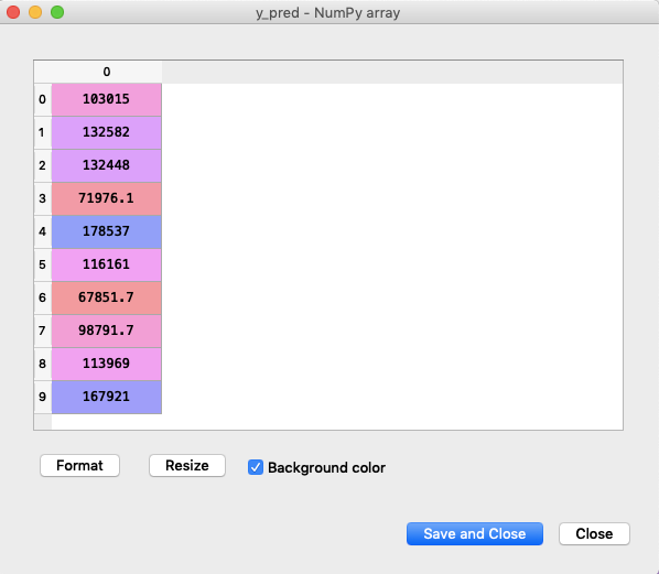
Now, let us compare the original and predicted values.
df1 = pd.DataFrame({'Actual': y_test.flatten(), 'Predicted': y_pred.flatten()})
df1.plot(kind='bar')
plt.grid(which='major', linestyle='-', linewidth='0.5', color='green')
plt.grid(which='minor', linestyle=':', linewidth='0.5', color='black')
plt.show()
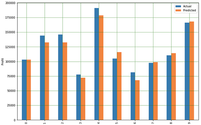
Not bad isn’t it, now since we have our model ready let’s fine-tune our model for better accuracy.
Now, its time to build an optimal regression model using Backward Elimination method.
3. Building the optimal model using Backward Elimination
Backward Elimination
The goal here is to build a high-quality multiple regression model that includes a few attributes as possible, without compromising the predictive ability of the model.
Steps involved in backward elimination:
Step-1: Select a Significance Level(SL) to stay in your model(SL = 0.05)
Step-2: Fit your model with all possible predictors.
Step-3: Consider the predictor with the highest p-value; if p-value>SL, go to Step-4: Otherwise model is ready.
Step-4: Remove the predictor.
Step-5: Fit the model without this variable.
Here, the significance level and p-value are statistical terms, just remember these terms for now as we do not want to go in details. Just note that our python libraries will provide us these values for our independent variables.
Coming back to our scenario, as we know that multiple linear regression is represented as :
y = b0 + b1X1 + b2X2 + b3X3 +…..+ bnXn
we can also represent it as
y = b0X0 + b1X1 + b2X2 + b3X3 +…..+ bnXn where X0 = 1
We have to add one column with all 50 values as 1 to represent b0X0.
import statsmodels.formula.api as smX = np.append(arr = np.ones((50,1)).astype(int), values = X, axis = 1)
statsmodels python library provides an OLS(ordinary least square) class for implementing Backward Elimination. Now one thing to note that OLS class does not provide the intercept by default and it has to be created by the user himself. That is why we created a column with all 50 values as 1 to representb0X0 in the previous step.
In the first step, let us create variable X_opt which will contain variables which are statistically significant(has maximum impact on the dependent variable) and for doing that we have to start with considering all the independent variables and in each step, we will remove variables with the maximum p-value.
X_opt = X[:,[0,1,2,3,4,5]]
regressor_OLS = sm.OLS(endog = y, exog = X_opt).fit()
regressor_OLS.summary()
Here endog means the dependent variable and exog means X_opt .
We can remove index x2 as it has the highest p-value.
Again repeat the process
X_opt = X[:,[0,1,3,4,5]]
regressor_OLS = sm.OLS(endog = y, exog = X_opt).fit()
regressor_OLS.summary()
We can remove index x1 as it has the highest p-value.
Again repeat the process
X_opt = X[:,[0,3,4,5]]
regressor_OLS = sm.OLS(endog = y, exog = X_opt).fit()
regressor_OLS.summary()
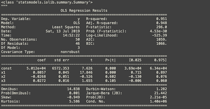
We can remove index x2 as it has the highest p-value.
Again repeat the process
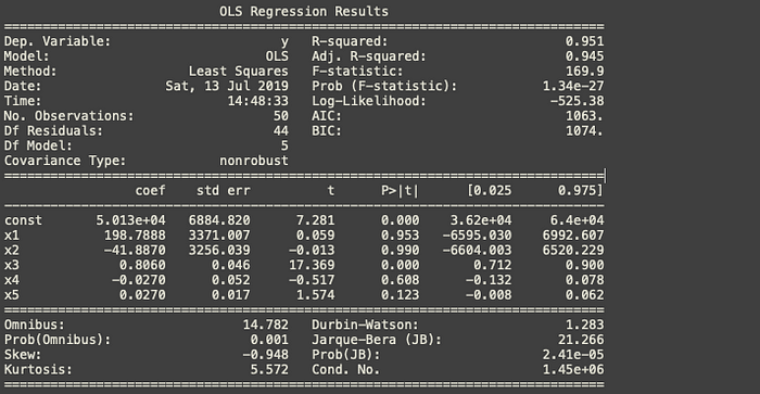
X_opt = X[:,[0,3,5]]
regressor_OLS = sm.OLS(endog = y, exog = X_opt).fit()
regressor_OLS.summary()
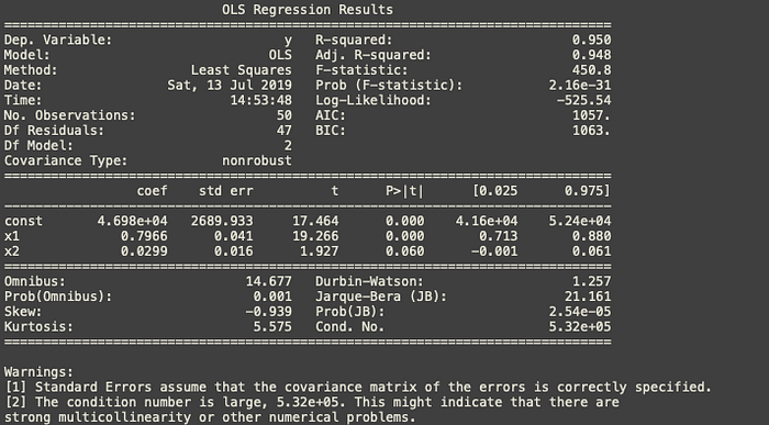
Now as per the rule we have to remove index x2 as it is more than the significance level but it should be considered as very close the significance level of 50%. But we will go ahead strictly with the rule and we’ll remove index x2. Hold onto this we will discuss this in the next section.
Again repeat the process
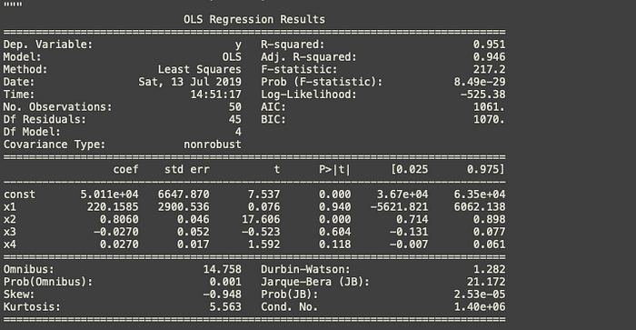
X_opt = X[:,[0,3]]
regressor_OLS = sm.OLS(endog = y, exog = X_opt).fit()
regressor_OLS.summary()
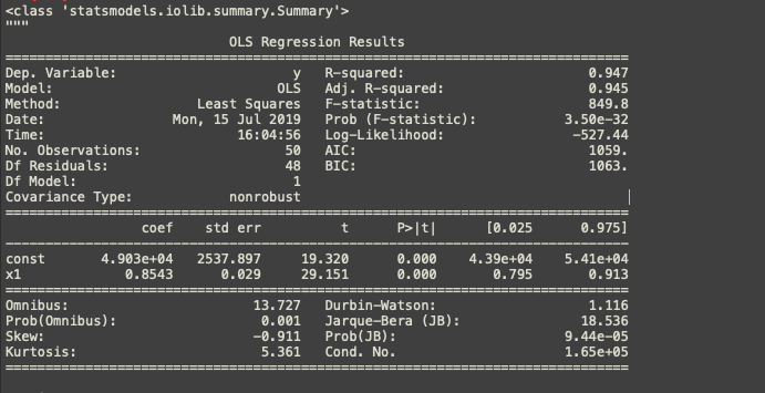
We have all the variables under the significance level of 0.05. It means, the only one variable left out i.e. x1(R&D spend) has the highest impact on the profit and is statistically significant.
Congratulations!!! We have just created an optimal regressor model using Backward Elimination method.
Now let’s make our model more robust by considering some more metrics like R-squared and Adj. R-squared.
4. Fine-tune our optimal Regressor Model
Before we start tuning our model lets get familiar with two important concepts.
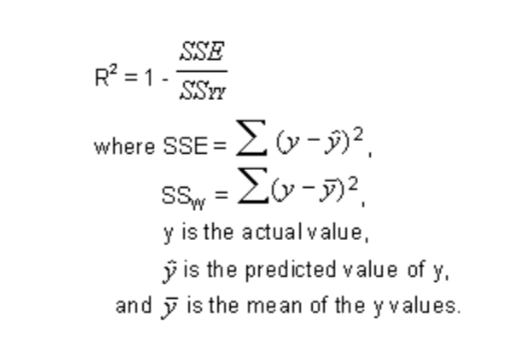
4.1) R-squared
It is a statistical measure of how close the data are to the fitted regression line. It is also known as the coefficient of determination or coefficient of multiple determination.
R-squared is always between 0 and 100%:
0% indicates that the model explains none of the variability of the response data around its mean.
100% indicates that the model explains all the variability of the response data around its mean.
In general, the higher the R-squared, the better the model fits your data.
There are 2 major problems with R-squared, first, if we add more predictors, R-squared will always increase because OLS will never let R-squared decrease when more predictors are added. Secondly, if a model has too many predictors and higher-order polynomials, it begins to model the random noise in the data. This is called overfitting and produces misleadingly high R-squared values and lesser ability to make predictions.
That is why we need Adjusted R-squared.
4.2) Adjusted R-squared
The adjusted R-squared compares the explanatory power of regression models that contain different numbers of predictors.
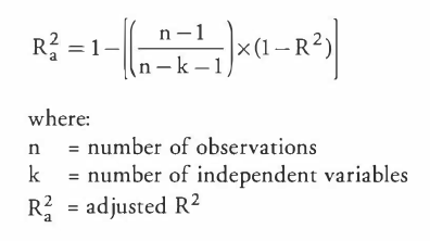
The adjusted R-squared is a modified version of R-squared that has been adjusted for the number of predictors in the model. The adjusted R-squared increases only if the new term improves the model more than would be expected by chance. It decreases when a predictor improves the model by less than expected by chance. The adjusted R-squared can be negative, but it’s usually not. It is always lower than the R-squared.
So coming back to our original model, there was a confusion in Result-4 whether to remove x2 or to retain it.
If Adjusted R-squared decreases with the addition of more predictors(and vice-versa) then our model fits better contrary to R-squared.
If we look closely to all the snapshots above, Adjusted R-squared is increasing till Result-4 but it decreased when the x2 was removed, see Result-5 which should not have happened.
Conclusion
So the final take away we have is the last step should not have been performed in the Backward Elimination method. We are left with R&D Spendand Marketing Spend as the final predictors.
X_opt = X[:,[0,3,5]]
This should be used as the matrix of independent variables instead of taking all the independent variables. Here, the index 0 represents a column of 1’s that we added.
That’s all in this article hope you guys have enjoyed reading this, let me know about your views/suggestions/questions in the comment section.
You can also reach me out over LinkedIn for any query.
Thanks for reading !!!
Bio: Nagesh Singh Chauhan is a Data Science enthusiast. Interested in Big Data, Python, Machine Learning.
Original. Reposted with permission.
Related:
- A Beginner’s Guide to Linear Regression in Python with Scikit-Learn
- Predict Age and Gender Using Convolutional Neural Network and OpenCV
- Classifying Heart Disease Using K-Nearest Neighbors