 Deep Learning for NLP: Creating a Chatbot with Keras!
 Deep Learning for NLP: Creating a Chatbot with Keras!
Learn how to use Keras to build a Recurrent Neural Network and create a Chatbot! Who doesn’t like a friendly-robotic personal assistant?
By Jaime Zornoza, Universidad Politecnica de Madrid

In the previous post, we learned what Artificial Neural Networks and Deep Learning are. Also, some neural network structures for exploiting sequential data like text or audio were introduced. If you haven’t read that post, you should sit back, grab a coffee, and slowly enjoy it. It can be found here.
This new post will cover how to use Keras, a very popular library for neural networks to build a Chatbot. The main concepts of this library will be explained, and then we will go through a step-by-step guide on how to use it to create a yes/no answering bot in Python. We will use the easy going nature of Keras to implement a RNN structure from the paper “End to End Memory Networks” by Sukhbaatar et al (which you can find here).
This is interesting because having defined a task or application (creating a yes/no chatbot to answer specific questions), we will learn how to translate the insights from a research work onto an actual model that we can then use to reach our application goals.
Don’t be scared if this is your first time implementing an NLP model; I will go through every step, and put a link to the code at the end. For the best learning experience, I suggest you first read the post, and then go through the code while glancing at the sections of the post that go along with it.
Lets get to it then!
Keras: Easy Neural Networks in Python
Keras is an open source, high level library for developing neural network models. It was developed by François Chollet, a Deep Learning researcher from Google. It’s core principle is to make the process of building a neural network, training it, and then using it to make predictions, easy and accessible for anyone with a basic programming knowledge, while still allowing developers to fully customise the parameters of the ANN.
Basically, Keras is actually just an interface that can run on top of different Deep Learning frameworks like CNTK, Tensorflow, or Theano for example. It works the same, independently of the back-end that is used.
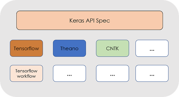
Layered structure of the Keras API. As it can be seen, it can run on top of different frameworks seamlessly.
As we mentioned in the previous post, in a Neural Network each node in a specific layer takes the weighted sum of the outputs from the previous layer, applies a mathematical function to them, and then passes that result to the next layer.
With Keras we can create a block representing each layer, where these mathematical operations and the number of nodes in the layer can be easily defined. These different layers can be created by typing an intuitive and single line of code.
The steps for creating a Keras model are the following:
Step 1: First we must define a network model, which most of the time will be the Sequential model: the network will be defined as a sequence of layers, each with its own customisable size and activation function. In these models the first layer will be the input layer, which requires us to define the size of the input that we will be feeding to the network. After this more and more layers can be added and customised until we reach the final output layer.
#Define Sequential Model
model = Sequential()
#Create input layer
model.add(Dense(32, input_dim=784))
#Create hidden layer
model.add(Activation('relu'))
#Create Output layer
model.add(Activation('sigmoid'))
Step 2: After creating the structure of the network in this manner we have to compile it, which transforms the simple sequence of layers that we have previously defined, into a complex group of matrix operations that dictate how the network behaves. Here we must define the optimisation algorithm that will be used to train the network, and also choose the loss function that will be minimised.
#Compiling the model with a mean squared error loss and RMSProp #optimizer
model.compile(optimizer='rmsprop',loss='mse')
Step 3: Once this is done, we can train or fit the network, which is done using the back-propagation algorithm mentioned in the previous post.
# Train the model, iterating on the data in batches of 32 samples model.fit(data, labels, epochs=10, batch_size=32)
Step 4: Hurray! Our network is trained. Now we can use it to make predictions on new data.
As you can see, it is fairly easy to build a network using Keras, so lets get to it and use it to create our chatbot! The blocks of code used above are not representative of an actual concrete neural network model, they are just examples of each of the steps to help illustrate how straightforward it is to build a Neural Network using the Keras API.
You can find all the documentation about Keras and how to install it in its official web page.
The Project: Using Recurrent Neural Networks to build a Chatbot
Now we know what all these different types of neural networks are, lets use them to build a chat-bot that can answer some questions for us!
Most of the time, neural network structures are more complex than just the standard input-hidden layer-output. Sometimes we might want to invent a neural network ourselfs and play around with the different node or layer combinations. Also, in some occasions we might want to implement a model we have seen somewhere, like in a scientific paper.
In this post we will go through an example of this second case, and construct the neural model from the paper “End to End Memory Networks” by Sukhbaatar et al (which you can find here).
Also we will see how to save the trained model, so that we don’t have to train the network every time we want to make predictions using the model we have built. Lets go then!
The model: Inspiration
As mentioned earlier, the RNN used in this post, has been taken from the paper “End to End Memory Networks” , so I recommend you take a look at it before proceeding, although I will explain the most relevant parts in the following lines.
This paper implements an RNN like structure that uses an attention model to compensate for the long term memory issue about RNNs that we discussed in the previous post.
Don’t know what an attention model is? Do not worry, I will explain it in simple terms to you. Attention models gathered a lot of interest because of their very good results in tasks like machine translation. They address the issue of long sequences and short term memory of RNNs that was mentioned previously.
To gather an intuition of what attention does, think of how a human would translate a long sentence from one language to another. Instead of taking the whoooooole sentence and then translating it in one go, you would split the sentence into smaller chunks and translate these smaller pieces one by one. We work part by part with the sentence because it is really difficult to memorise it entirely and then translate it at once.

An attention mechanism does just this. In each time step, the model gives a higher weight in the output to those parts of the input sentence that are more relevant towards the task that we are trying to complete. This is where the name comes from: it plays attention to what is more important. The example above illustrates this very well; to translate the first part of the sentence, it makes little sense to be looking at the entire sentence or to the last part of the sentence.
The following figure shows the performance of RNN vs Attention models as we increase the length of the input sentence. When faced with a very long sentence, and ask to perform a specific task, the RNN, after processing all the sentence will have probably forgotten about the first inputs it had.

Okay, now that we know what an attention model is, lets take a loser look at the structure of the model we will be using. This model takes an input xi (a sentence), a query q about such sentence, and outputs a yes/ no answer a.

On the left part of the previous image we can see a representation of a single layer of this model. Two different embeddings are calculated for each sentence, A and C. Also, the query or question q is embedded, using the B embedding.
The A embeddings mi, are then computed using an inner product with the question embedding u (this is the part where the attention is taking place, as by computing the inner product between these embeddings what we are doing is looking for matches of words from the query and the sentence, to then give more importance to these matches using a Softmax function on the resulting terms of the dot product).
Lastly, we compute the output vector o using the embeddings from C (ci), and the weights or probabilities pi obtained from the dot product. With this output vector o, the weight matrix W, and the embedding of the question u, we can finally calculate the predicted answer a hat.
To build the entire network, we just repeat these procedure on the different layers, using the predicted output from one of them as the input for the next one. This is shown on the right part of the previous image.
Don’t worry if all these came too quick at you, hopefully you will get a better and complete understanding as we go through the different steps to implement this model in Python.
The data: Stories, questions and answers
In 2015, Facebook came up with a bAbI data-set and 20 tasks for testing text understanding and reasoning in the bAbI project. The tasks are described in detail in the paper here.
The goal of each task is to challenge a unique aspect of machine-text related activities, testing different capabilities of learning models. In this post we will face one of these tasks, specifically the “QA with single supporting fact”.
The block bellow shows an example of the expected behaviour from this kind of QA bot:
FACT: Sandra went back to the hallway. Sandra moved to the office. QUESTION: Is Sandra in the office?ANSWER: yes
The data-set comes already separated into training data (10k instances) and test data (1k instances), where each instance has a fact, a question, and a yes/no answer to that question.
Now that we have seen the structure of our data, we need to build a vocabularyout of it. On a Natural Language Processing model a vocabulary is basically a set of words that the model knows and therefore can understand. If after building a vocabulary the model sees inside a sentence a word that is not in the vocabulary, it will either give it a 0 value on its sentence vectors, or represent it as unknown.
VOCABULARY:
'.', '?', 'Daniel', 'Is', 'John', 'Mary', 'Sandra', 'apple','back','bathroom', 'bedroom', 'discarded', 'down','dropped','football', 'garden', 'got', 'grabbed', 'hallway','in', 'journeyed', 'kitchen', 'left', 'milk', 'moved','no', 'office', 'picked', 'put', 'the', 'there', 'to','took', 'travelled', 'up', 'went', 'yes'
As our training data is not very varied (most questions use the same verbs and nouns but with different combinations), our vocabulary is not very big, but in moderately sized NLP projects the vocabulary can be very large.
Take into account that to build a vocabulary we should only use the training data most of the time; the test data should be separated from the training data at the very beginning of a Machine Learning project and not touched until it is time to asses the performance on the model that has been chosen and tuned.
After building the vocabulary we need to vectorize our data. As we are using normal words as the inputs to our models and computers can only deal with numbers under the hood, we need a way to represent our sentences, which are groups of words, as vectors of numbers. Vectorizing does just this.
There are many ways of vectorizing our sentences, like Bag of Words models, or Tf-Idf, however, for simplicity, we are going to just use an indexing vectorizing technique, in which we give each of the words in the vocabulary a unique index from 1 to the length of the vocabulary.
VECTORIZATION INDEX:
'the': 1, 'bedroom': 2, 'bathroom': 3, 'took': 4, 'no': 5, 'hallway': 6, '.': 7, 'went': 8, 'is': 9, 'picked': 10, 'yes': 11, 'journeyed': 12, 'back': 13, 'down': 14, 'discarded': 15, 'office': 16, 'football': 17, 'daniel': 18, 'travelled': 19, 'mary': 20, 'sandra': 21, 'up': 22, 'dropped': 23, 'to': 24, '?': 25, 'milk': 26, 'got': 27, 'in': 28, 'there': 29, 'moved': 30, 'garden': 31, 'apple': 32, 'grabbed': 33, 'kitchen': 34, 'put': 35, 'left': 36, 'john': 37}
Take into account that this vectorization is done using a random seed to start, so even tough you are using the same data as me, you might get different indexes for each word. Don’t worry; this will not affect the results of the project. Also, the words in our vocabulary were in upper and lowercase; when doing this vectorization all the words get lowercased for uniformity.
After this, because of the way Keras works, we need to pad the sentences. What does this mean? It means that we need to search for the length of the longest sentence, convert every sentence to a vector of that length, and fill the gap between the number of words of each sentence, and the number of words of the longest sentences with zeros.
After doing this, a random sentence of the dataset should look like:
FIRST TRAINING SENTENCE VECTORIZED AND PADDED:
array([ 0,  0,  0,  0,  0,  0,  0,  0,  0,  0,  0,  0,  0,  0,  0,  0,  0,
        0,  0,  0,  0,  0,  0,  0,  0,  0,  0,  0,  0,  0,  0,  0,  0,  0,
        0,  0,  0,  0,  0,  0,  0,  0,  0,  0,  0,  0,  0,  0,  0,  0,  0,
        0,  0,  0,  0,  0,  0,  0,  0,  0,  0,  0,  0,  0,  0,  0,  0,  0,
        0,  0,  0,  0,  0,  0,  0,  0,  0,  0,  0,  0,  0,  0,  0,  0,  0,
        0,  0,  0,  0,  0,  0,  0,  0,  0,  0,  0,  0,  0,  0,  0,  0,  0,
        0,  0,  0,  0,  0,  0,  0,  0,  0,  0,  0,  0,  0,  0,  0,  0,  0,
        0,  0,  0,  0,  0,  0,  0,  0,  0,  0,  0,  0,  0,  0,  0,  0,  0,
        0,  0,  0,  0,  0,  0,  0,  0, 20, 30, 24,  1,  3,  7, 21, 12, 24, 1,  2,  7])
As we can see, it has zeros everywhere except in the end (this sentence was a lot shorter than the longest sentence), where it has some numbers. What are these numbers? Well, they are the indexes representing the different words of the sentence: 20 is the index representing the word Mary, 30 is moved, 24 is to, 1 is the, 3 represents bathroom and so on. The actual sentence is:
FIRST TRAINING SENTENCE:
"Mary moved to the bathroom . Sandra journeyed to the bedroom ."
Okay, now that we have prepared the data, we are ready to build our Neural Network!
The Neural Network: Building the model
The first step to creating the network is to create what in Keras is known as placeholders for the inputs, which in our case are the stories and the questions. In an easy manner, these placeholders are containers where batches of our training data will be placed before being fed to the model.
#Example of a Placeholder
question = Input((max_question_len,batch_size))
They have to have the same dimension as the data that will be fed, and can also have a batch size defined, although we can leave it blank if we dont know it at the time of creating the placeholders.
Now we have to create the embeddings mentioned in the paper, A, C and B. An embedding turns an integer number (in this case the index of a word) into a ddimensional vector, where context is taken into account. Word embeddings arewidely used in NLP and is one of the techniques that has made the field progress so much in the recent years.
#Create input encoder A:
input_encoder_m = Sequential()
input_encoder_m.add(Embedding(input_dim=vocab_len,output_dim = 64))
input_encoder_m.add(Dropout(0.3))#Outputs: (Samples, story_maxlen,embedding_dim) -- Gives a list of #the lenght of the samples where each item has the
#lenght of the max story lenght and every word is embedded in the embbeding dimension
The code above is an example of one of the embeddings done in the paper (A embedding). Like always in Keras, we first define the model (Sequential), and then add the embedding layer and a dropout layer, which reduces the chance of the model over-fitting by triggering off nodes of the network.
Once we have created the two embeddings for the input sentences, and the embeddings for the questions, we can start defining the operations that take place in our model. As mentioned previously, we compute the attention by doing the dot product between the embedding of the questions and one of the embeddings of the stories, and then doing a softmax. The following block shows how this is done:
match = dot([input_encoded_m,question_encoded], axes = (2,2))
match = Activation('softmax')(match)
After this, we need to calculate the output o adding the match matrix with the second input vector sequence, and then calculate the response using this output and the encoded question.
response = add([match,input_encoded_c])
response = Permute((2,1))(response)
answer = concatenate([response, question_encoded])
Lastly, once this is done we add the rest of the layers of the model, adding an LSTM layer (instead of an RNN like in the paper), a dropout layer and a final softmax to compute the output.
answer = LSTM(32)(answer)
answer = Dropout(0.5)(answer)
#Output layer:
answer = Dense(vocab_len)(answer)
#Output shape: (Samples, Vocab_size) #Yes or no and all 0s
answer = Activation('softmax')(answer)
Notice here that the output is a vector of the size of the vocabulary (that is, the length of the number of words known by the model), where all the positions should be zero except the ones at the indexes of ‘yes’ and ‘no’.
Learning from the data: Training the model
Now we are ready to compile the model, and train it!
model = Model([input_sequence,question], answer)
model.compile(optimizer='rmsprop', loss = 'categorical_crossentropy', metrics = ['accuracy'])
With these two lines we build the final model, and compile it, that is, define all the maths that will be going on in the background by specifying an optimiser, a loss function and a metric to optimise.
Now its time to train the model, here we need to define the inputs to the training, (the input stories, questions and answers), the batch size that we will be feeding the model with (that is, how many inputs at once), and the number of epochs that we will train the model for (that is, how many times the model will go through the training data in order to update the weights). I used 1000 epochs and obtained an accuracy of 98%, but even with 100 to 200 epochs you should get some pretty good results.
Note that depending on your hardware, this training might take a while. Just relax, sit back, keep reading Medium and wait until its done.
After its completed the training you might be left wondering “am I going to have to wait this long every time I want to use the model?” the obvious answer my friend is, NO. Keras allows developers to save a certain model it has trained, with the weights and all the configurations. The following block of code shows how this is done.
filename = 'medium_chatbot_1000_epochs.h5'
model.save(filename)
Now, when we want to use the model is as easy as loading it like so:
model.load_weights('medium_chatbot_1000_epochs.h5')
Cool cool. Now that we have trained our model, lets see how it performs on new data, and play a little bit with it!
Seeing the results: Testing and playing
Lets see how our model performs on the test data!
pred_results = model.predict(([inputs_test,questions_test]))
These results are an array, as mentioned earlier that contain in every position the probabilities of each of the words in the vocabulary being the answer to the question. If we look at the first element of this array, we will see a vector of the size of the vocabulary, where all the times are close to 0 except the ones corresponding to yes or no.
Out of these, if we pick the index of the highest value of the array and then see to which word it corresponds to, we should find out if the answer is affirmative or negative.
One fun thing that we can do now, is create our own stories and questions, and feed them to the bot to see what he says!
my_story = 'Sandra picked up the milk . Mary travelled left . '
my_story.split()
my_question = 'Sandra got the milk ?'
my_question.split()
I created a story and a question somehow similar to what our little bot has seen before, and after adapting it to the format that the neural network wants the bot answered ‘YES’ (in lowercase tough, he is not as enthusiastic as I am).
Let's try with something different:
my_story = 'Medium is cool . Jaime really likes it. '
my_story.split()
my_question = 'Does Jaime like Medium ?'
my_question.split()
The answer this time was: ‘Of course, who doesn’t?’
Just kidding, I didn’t try that story/question combination, as many of the words included are not inside the vocabulary of our little answering machine. Also, he only knows how to say ‘yes’ and ‘no’, and does not usually give out any other answers. However, with more training data and some workarounds this could be easily achieved.
That is it for today! I hope you guys enjoyed reading the post as much as I enjoyed writing it. Have a good day, take care, and enjoy AI!
You can find the code and the data on my Github page.
Other resources:
If you want to go deeper into attention models, or understand some word vectorizing techniques that I mentioned, check out these additional resources I’ve put together for you. Enjoy!
A Beginner’s Guide to Attention Mechanisms and Memory Networks
Andrew’s Ng video with the intuition to attention models.
A Begginner’s Guide to Tf-Idf and Bag of Words.
Keras guide to building this same model.
Feel Free to connect with me on LinkedIn or follow me on Twitter at @jaimezorno. Also, you can take a look at my other posts on Data Science and Machine Learning here. Have a good read!
Bio: Jaime Zornoza is an Industrial Engineer with a bachelor specialized in Electronics and a Masters degree specialized in Computer Science.
Original. Reposted with permission.
Related:
- Deep Learning for NLP: ANNs, RNNs and LSTMs explained!
- Training a Neural Network to Write Like Lovecraft
- Adapters: A Compact and Extensible Transfer Learning Method for NLP