Detecting stationarity in time series data
Explore how to determine if your time series data is generated by a stationary process and how to handle the necessary assumptions and potential interpretations of your result.
By Shay Palachy, Data Science Consultant.
Stationarity is an important concept in time series analysis. For a concise (but thorough) introduction to the topic, and the reasons that make it important, take a look at my previous blog post on the topic. Without reiterating too much, it suffices to say that:
- Stationarity means that the statistical properties of a time series (or rather the process generating it) do not change over time.
- Stationarity is important because many useful analytical tools and statistical tests and models rely on it.
As such, the ability to determine if a time series is stationary is important. Rather than deciding between two strict options, this usually means being able to ascertain, with high probability, that a series is generated by a stationary process.
In this brief post, I will cover several ways to do just that.
Visualizations
The most basic methods for stationarity detection rely on plotting the data, or functions of it, and determining visually whether they present some known property of stationary (or non-stationary) data.
Looking at the data
Trying to determine whether a time series was generated by a stationary process just by looking at its plot is a dubious venture. However, there are some basic properties of non-stationary data that we can look for. Let’s take as an example the following nice plots from [Hyndman & Athanasopoulos, 2018]:
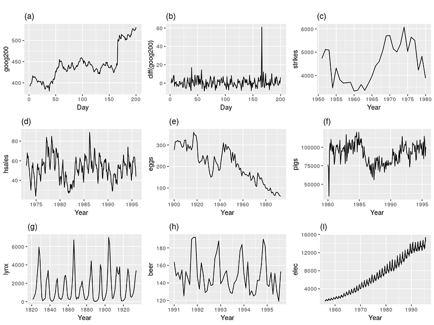
Figure 1. Nine examples of time series data; (a) Google stock price for 200 consecutive days; (b) Daily change in the Google stock price for 200 consecutive days; (c) Annual number of strikes in the US; (d) Monthly sales of new one-family houses sold in the US; (e) Annual price of a dozen eggs in the US (constant dollars); (f) Monthly total of pigs slaughtered in Victoria, Australia; (g) Annual total of lynx trapped in the McKenzie River district of north-west Canada; (h) Monthly Australian beer production; (i) Monthly Australian electricity production. [Hyndman & Athanasopoulos, 2018]
[Hyndman & Athanasopoulos, 2018] give several heuristics used to rule out stationarity in the above plots, corresponding to the basic characteristic of stationary processes (which we’ve discussed previously):
- Prominent seasonality can be observed in series (d), (h) and (i).
- Noticeable trends and changing levels can be seen in series (a), (c), (e), (f), and (i).
- Series (i) shows increasing variance.
The authors also add that although the strong cycles in series (g) might appear to make it non-stationary, the timing of these cycles makes them unpredictable (due to the underlying dynamic dominating lynx population, driven partially by available feed). This leaves series (b) as the only stationary series.
If like me, you didn’t find at least some of these observations trivial to make by looking at the above figure, you are not the only one. Indeed, this is not a very dependable method to detect stationarity, and it is usually used to get an initial impression of the data rather than to make definite assertions.
Looking at Autocorrelation Function (ACF) plots
Autocorrelation is the correlation of a signal with a delayed copy — or a lag — of itself as a function of the delay. When plotting the value of the ACF for increasing lags (a plot called a correlogram), the values tend to degrade to zero quickly for stationary time series (see figure 1, right), while for non-stationary data the degradation will happen more slowly (see figure 1, left).
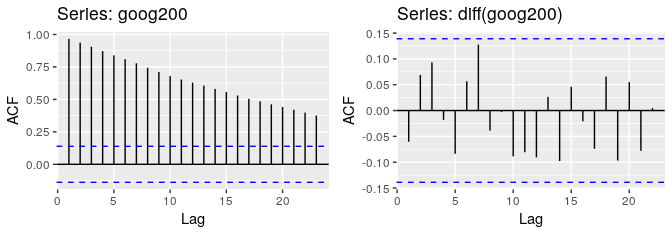
Figure 2. The ACF of the Google stock price (left; non-stationary), and of the daily changes in Google stock price (right; stationary).
Alternatively, [Nielsen, 2006] suggests that plotting correlograms based on both autocorrelations and scaled autocovariances, and comparing them, provides a better way of discriminating between stationary and non-stationary data.
Parametric tests
Another, more rigorous approach, to detecting stationarity in time series data is using statistical tests developed to detect specific types of stationarity, namely those brought about by simple parametric models of the generating stochastic process (see my previous post for details).
I’ll present here the most prominent tests. I’ll also name Python implementations for each test, assuming I have found any. For R implementations, see the CRAN Task View: Time Series Analysis (also here).
Unit root tests
The Dickey-Fuller Test
The Dickey-Fuller test was the first statistical test developed to test the null hypothesis that a unit root is present in an autoregressive model of a given time series and that the process is thus not stationary. The original test treats the case of a simple lag-1 AR model. The test has three versions that differ in the model of unit root process they test for;
- Test for a unit root: ∆yᵢ = δyᵢ₋₁ + uᵢ
- Test for a unit root with drift: ∆yᵢ = a₀ + δyᵢ₋₁ + uᵢ
- Test for a unit root with drift and deterministic time trend:
∆yᵢ = a₀ + a₁*t + δyᵢ₋₁ + uᵢ
The choice of which version to use — which can significantly affect the size and power of the test — can use prior knowledge or structured strategies for series of ordered tests, allowing the discovery of the most fitting version.
Extensions of the test were developed to accommodate more complex models and data; these include the Augmented Dickey-Fuller (ADF) (using AR of any order p and supporting modeling of time trends), the Phillips-Perron test (PP) (adding robustness to unspecified autocorrelation and heteroscedasticity)and the ADF-GLS test (locally de-trending data to deal with constant and linear trends).
Python implementations can be found in the statsmodels and ARCH packages.
The KPSS Test
Another prominent test for the presence of a unit root is the KPSS test. [Kwiatkowski et al., 1992] Conversely to the Dickey-Fuller family of tests, the null hypothesis assumes stationarity around a mean or a linear trend, while the alternative is the presence of a unit root.
The test is based on linear regression, breaking up the series into three parts: a deterministic trend (βt), a random walk (rt), and a stationary error (εt), with the regression equation:
![]()
where u~(0,σ²) and are iid. The null hypothesis is thus stated to be H₀: σ²=0 while the alternative is Hₐ: σ²>0. Whether the stationarity in the null hypothesis is around a mean or a trend is determined by setting β=0 (in which case x is stationary around the mean r₀) or β≠0, respectively.
The KPSS test is often used to complement Dickey-Fuller-type tests. I will touch on how to interpret such combined results in a future post.
Python implementations can be found in the statsmodels and ARCH packages.
The Zivot and Andrews Test
The tests above do not allow for the possibility of a structural break — an abrupt change involving a change in the mean or other parameters of the process. Assuming the time of the break as an exogenous phenomenon, Perron showed that the power to reject a unit root decreases when the stationary alternative is true and a structural break is ignored.
[Zivot and Andrews, 1992] propose a unit root test in which they assume that the exact time of the break-point is unknown. Following Perron’s characterization of the form of a structural break, Zivot and Andrews proceed with three models to test for a unit root:
- Model A: Permits a one-time change in the level of the series.
- Model B: Allows for a one-time change in the slope of the trend function.
- Model C: Combines one-time changes in the level and the slope of the trend function of the series.
Hence, to test for a unit root against the alternative of a one-time structural break, Zivot and Andrews use the following regression equations corresponding to the above three models [Waheed et al., 2006]:
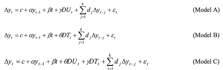
A Python implementation can be found in the ARCH package and here.
Semi-parametric unit root tests
Variance Ratio Test
[Breitung, 2002] suggested a non-parametric test for the presence of a unit root based on a variance ratio statistic. The null hypothesis is a process I(1) (integrated of order one) while the alternative is I(0). I list this test as semi-parametric because it tests for a specific, model-based, notion of stationarity.
Non-parametric tests
In the wake of the limitations of parametric tests, and the recognition they cover only a narrow sub-class of possible cases encountered in real data, a class of non-parametric tests for stationarity has emerged in time series analysis literature.
Naturally, these tests open up a promising avenue for investigating time series data: you no longer have to assume very simple parametric models happen to apply to your data to find out whether it is stationary or not, or risk not discovering a complex form of the phenomenon not captured by these models.
The reality of it, however, is more complex; there aren’t, at the moment, any widely-applicable non-parametric tests that encompass all real-life scenarios generating time series data. Instead, these tests limit themselves to specific types of data or processes. Also, I was not able to find implementations for any of the following tests.
I’ll mention here the few that I have encountered:
A Nonparametric Test for Stationarity in Continuous-Time Markov Processes
[Kanaya, 2011] suggest this nonparametric test stationarity for univariate time-homogeneous Markov processes only, construct a kernel-based test statistic and conduct Monte-Carlo simulations to study the finite-sample size and power properties of the test.
A nonparametric test for stationarity in functional time series
[Delft et al., 2017] suggest a nonparametric stationarity test limited to functional time series — data obtained by separating a continuous (in nature) time record into natural consecutive intervals, for example, days. Note that [Delft and Eichler, 2018] have proposed a test for local stationarity for functional time series (see my previous post for some references on local stationarity). Also, [Vogt & Dette, 2015] suggest a nonparametric method to estimate a smooth change point in a locally stationary framework.
A nonparametric test for stationarity based on local Fourier analysis
[Basu et al., 2009] suggest what may be the most applicable nonparametric test for stationarity present here, as it applies to any zero-mean discrete-time random process (and I assume here any finite sample of a discrete process you may have can easily be transformed to have zero mean).
Final Words
That’s it. I hope the above review gave some idea as to how to approach the issue of detecting stationarity in your data. I also hope that it exposed you to the complexities of this task; due to the lack of implementations to the handful of nonparametric tests out there, you will be forced to make strong assumptions about your data, and interpret the results you get with the required amount of doubt.
As to the question of what to do once who have detected some stationarity in your data, I hope to touch on this in a future post. As always, I’d love to hear about things I’ve missed or was wrong about. Cheers!
References
Academic literature
- Basu, P., Rudoy, D., & Wolfe, P. J. (2009, April). A nonparametric test for stationarity based on local Fourier analysis. In 2009 IEEE International Conference on Acoustics, Speech and Signal Processing(pp. 3005–3008). IEEE.
- Breitung, J. (2002). Nonparametric tests for unit roots and cointegration. Journal of econometrics, 108(2), 343–363.
- Cardinali, A., & Nason, G. P. (2018). Practical powerful wavelet packet tests for second-order stationarity. Applied and Computational Harmonic Analysis, 44(3), 558–583.
- Hyndman, R. J., & Athanasopoulos, G. (2018). Forecasting: principles and practice. OTexts.
- Kanaya, S. (2011). A nonparametric test for stationarity in continuous & time markov processes. Job Market Paper, University of Oxford.
- Kwiatkowski, D., Phillips, P. C., Schmidt, P., & Shin, Y. (1992). Testing the null hypothesis of stationarity against the alternative of a unit root: How sure are we that economic time series have a unit root? Journal of econometrics, 54(1–3), 159–178.
- Nielsen, B. (2006). Correlograms for non‐stationary autoregressions. Journal of the Royal Statistical Society: Series B (Statistical Methodology), 68(4), 707–720.
- Waheed, M., Alam, T., & Ghauri, S. P. (2006). Structural breaks and unit root: evidence from Pakistani macroeconomic time series. Available at SSRN 963958.
- van Delft, A., Characiejus, V., & Dette, H. (2017). A nonparametric test for stationarity in functional time series. arXiv preprint arXiv:1708.05248.
- van Delft, A., and Eichler, M. (2018). “Locally stationary functional time series.” Electronic Journal of Statistics, 12:107–170.
- Vogt, M., & Dette, H. (2015). Detecting gradual changes in locally stationary processes. The Annals of Statistics, 43(2), 713–740.
- Zivot, E. and D. Andrews, (1992), Further evidence of great crash, the oil price shock and unit root hypothesis, Journal of Business and Economic Statistics,10, 251–270.
Online references
- Data transformations and forecasting models: what to use and when
- Forecasting Flow Chart
- Documentation of the egcm R package
- “Non-Stationary Time Series and Unit Root Tests” by Heino Bohn Nielsen
- How to interpret Zivot & Andrews unit root test?
Original. Reposted with permission.
Bio: Shay Palachy works as a machine learning and data science consultant after being the Lead Data Scientist of ZenCity, a data scientist at Neura, and a developer at Intel and Ravello (now Oracle Cloud). Shay also founded and manages NLPH, an initiative meant to encourage open NLP tools for Hebrew.
Related: