How (not) to use Machine Learning for time series forecasting: Avoiding the pitfalls

We outline some of the common pitfalls of machine learning for time series forecasting, with a look at time delayed predictions, autocorrelations, stationarity, accuracy metrics, and more.

comments

By Vegard Flovik.

In my other posts, I have covereaud topics such as: How to combine machine learning and physics, and how machine learning can be used for production optimization as well as anomaly detection and condition monitoring. But in this post, I will discuss some of the common pitfalls of machine learning for time series forecasting.

Time series forecasting is an important area of machine learning. It is important because there are so many prediction problems that involve a time component. However, while the time component adds additional information, it also makes time series problems more difficult to handle compared to many other prediction tasks.

This post will go through the task of time series forecasting using machine learning, and how to avoid some of the common pitfalls. Through a concrete example, I will demonstrate how one could seemingly have a good model and decide to put it into production, whereas in reality, the model might have no predictive power whatsoever, More specifically, I will focus on how to evaluate your model accuracy, and show how relying simply on common error metrics such as mean percentage error, R2 score etc. can be very misleading if they are applied without caution.

Machine learning models for time series forecasting

There are several types of models that can be used for time-series forecasting. In this specific example, I used a Long short-term memory network, or in short LSTM Network, which is a special kind of neural network that make predictions according to the data of previous times. It is popular for language recognition, time series analysis and much more. However, in my experience, simpler types of models actually provide just as accurate predictions in many cases. Using models such as e.g. random forest, gradient boosting regressorand time delay neural networks, temporal information can be included through a set of delays that are added to the input, so that the data is represented at different points in time. Due to their sequential nature, TDNN’s are implemented as a feedforward neural network instead of a recurrent neural network.

How to implement the models using open source software libraries

I usually define my neural network type of models using Keras, which is a high-level neural networks API, written in Python and capable of running on top of TensorFlow, CNTK, or Theano. For other types of models I usually use Scikit-Learn, which is a free software machine learning library, It features various classification, regression and clustering algorithms including support vector machines, random forests, gradient boosting, k-means and DBSCAN, and is designed to inter-operate with the Python numerical and scientific libraries NumPy and SciPy.

However, the main topic of this article is not how to implement a time series forecasting model, but rather how to evaluate the model predictions. Due to this, I will not go into the details of model building etc., as there are plenty of other blog posts and articles covering those subjects.

Example case: Prediction of time series data

The example data used in this case is illustrated in the figure below. I will get back to the data in more detail later, but for now, let`s assume this data represents e.g. the yearly evolution of a stock index. The data is split into a training and test set where the first 250 days are used as training data for the model, and we then try to predict the stock index during the last part of the dataset.

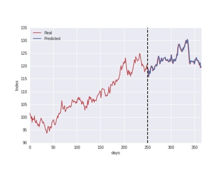
As I do not focus on model implementation in this article, let`s proceed directly to the process of evaluating the model accuracy. Just by visually inspecting the above figure, the model predictions seem to follow the real index closely, indicating a good accuracy. However, to be a bit more precise, we can evaluate the model accuracy by plotting the real vs. predicted values in a scatter plot as illustrated below, and also calculate the common error metric R2 score.

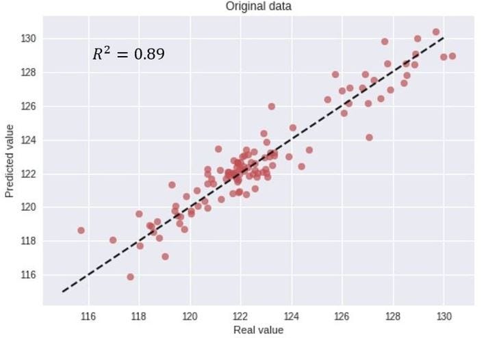
From the model predictions, we obtain an R2 score of 0.89, and seemingly a good match between the real and predicted values. However, as I will now discuss in more detail, this metric and model evaluation can be very misleading.

This is simply WRONG….

From the above figures and calculated error metrics, the model is apparently giving accurate predictions. However, this is not the case at all, and is simply an example of how choosing the wrong accuracy metric can be very misleading when evaluating model performance. In this example, for the sake of illustration, the data was explicitly chosen to represent data that actually cannot be predicted. More specifically, the data I called “stock index”, was actually modeled using a random walk process. As the name indicates, a random walk is a completely stochastic process. Due to this, the idea of using historical data as a training set in order to learn the behavior and predict future outcomes is simply not possible. Given this, how could it then be that the model is seemingly giving us such accurate predictions? As I will get back to in more detail, it all comes down to the (wrong) choice of accuracy metric.

Time delayed predictions and autocorrelations

Time series data, as the name indicates, differ from other types of data in the sense that the temporal aspect is important. On a positive note, this gives us additional information that can be used when building our machine learning model, that not only the input features contain useful information, but also the changes in input/output over time. However, while the time component adds additional information, it also makes time series problems more difficult to handle compared to many other prediction tasks.

In this specific example, I used an LSTM Network that make predictions according to the data at previous times. However, when zooming in a bit on the model predictions, as indicated in the figure below, we start to see what the model is actually doing.

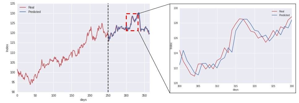
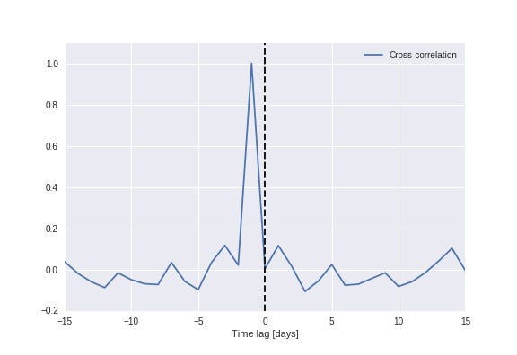
Time series data tend to be correlated in time, and exhibit a significant autocorrelation. In this case, that means that the index at time “t+1” is quite likely close to the index at time “t”. As illustrated in the above figure to the right, what the model is actually doing is that when predicting the value at time “t+1”, it simply uses the value at time “t” as its prediction (often referred to as the persistence model). Plotting the cross-correlation between the predicted and real value (below figure), we see a clear peak at a time lag of 1 day, indicating that the model simply uses the previous value as the prediction for the future.

Accuracy metrics can be very misleading when used incorrectly

This means that when evaluating the model in terms of its ability of predicting the value directly, common error metrics such as mean percentage error and R2 score both indicate a high prediction accuracy. However, as the example data is generated through a random walk process, the model cannot possibly predict future outcomes. This underlines the important fact that simply evaluating the models predictive powers through directly calculating common error metrics can be very misleading, and one can easily be fooled into being overly confident in the model accuracy.

Stationarity and differencing time series data

A stationary time series is one whose statistical properties such as mean, variance, autocorrelation, etc. are all constant over time. Most statistical forecasting methods are based on the assumption that the time series can be rendered approximately stationary (i.e., “stationarized”) through the use of mathematical transformations. One such basic transformation, is to time-difference the data, as illustrated in the below figure.

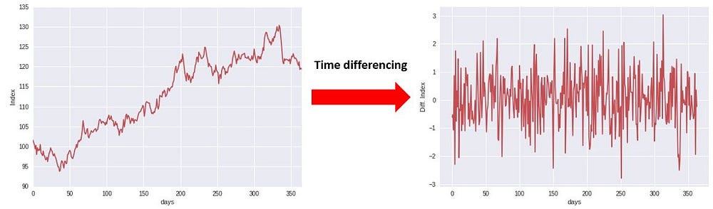
What this transformation does, is that rather than considering the index directly, we are calculating the difference between consecutive time steps.

Defining the model to predict the difference in values between time steps rather than the value itself, is a much stronger test of the models predictive powers. In that case, it cannot simply use that the data has a strong autocorrelation, and use the value at time “t” as the prediction for “t+1”. Due to this, it provides a better test of the model and if it has learnt anything useful from the training phase, and whether analyzing historical data can actually help the model predict future changes.

Prediction model for time-differenced data

As being able to predict the time-differenced data, rather than the data directly, is a much stronger indication of the predictive power of the model, let us try this with our model. The results of this test are illustrated in the figure below, showing a scatter-plot of the real vs. predicted values.

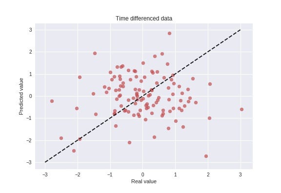
This figure indicates that the model is not able to predict future changes based on historical events, which is the expected result in this case, since the data is generated using a completely stochastic random walk process. Being able to predict future outcomes of a stochastic process is by definition not possible, and if someone claims to do this, one should be a bit skeptical…

Is your time series a random walk?

Your time series may actually be a random walk, and some ways to check this are as follows:

The time series shows a strong temporal dependence (autocorrelation) that decays linearly or in a similar pattern.
The time series is non-stationary and making it stationary shows no obviously learnable structure in the data.
The persistence model (using the observation at the previous time step as what will happen in the next time step) provides the best source of reliable predictions.

This last point is key for time series forecasting. Baseline forecasts with the persistence model quickly indicate whether you can do significantly better. If you can’t, you’re probably dealing with a random walk (or close to it). The human mind is hardwired to look for patterns everywhere and we must be vigilant that we are not fooling ourselves and wasting time by developing elaborate models for random walk processes.

Author note: after publishing the article I became aware of a nice article on the same topic by Jason Brownlee, which has similar treatment of random walks and time series: A Gentle Introduction to the Random Walk for Times Series Forecasting with Python.

Summary

The main point I would like to emphasize through this article, is to be very careful when evaluating your model performance in terms of prediction accuracy. As shown through the above example, even for a completely random process, where predicting future outcomes is by definition impossible, one can easily be fooled. By simply defining a model, making some predictions and calculating common accuracy metrics, one could seemingly have a good model and decide to put it into production. Whereas, in reality, the model might have no predictive power whatsoever.

If you are working with time series forecasting, and perhaps consider yourself a Data Scientist, I would urge you to put an emphasis on the Scientist aspect as well. Always be skeptical to what the data is telling you, ask critical questions and never draw any rash conclusions. The scientific method should be applied in data science as in any other kind of science.

Original. Reposted with permission.

Bio: Vegard Flovik is a Lead Data Scientist. Machine learning and advanced analytics at Axbit AS.

Resources:

Related:

How (not) to use Machine Learning for time series forecasting: Avoiding the pitfalls

Machine learning models for time series forecasting

How to implement the models using open source software libraries