Designing Your Neural Networks
Check out this step-by-step walk through of some of the more confusing aspects of neural nets to guide you to making smart decisions about your neural network architecture.
By Lavanya Shukla, Weights and Biases.

Training neural networks can be very confusing!
What’s a good learning rate? How many hidden layers should your network have? Is dropout actually useful? Why are your gradients vanishing?
In this post, we’ll peel the curtain behind some of the more confusing aspects of neural nets, and help you make smart decisions about your neural network architecture.
I highly recommend forking this kernel and playing with the different building blocks to hone your intuition.
If you have any questions, feel free to message me. Good luck!
1. Basic Neural Network Structure
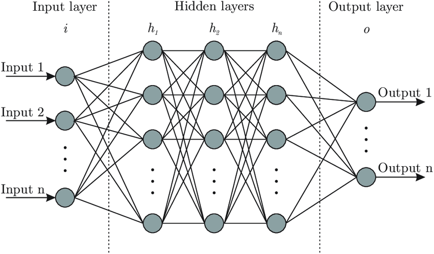
Input neurons
- This is the number of features your neural network uses to make its predictions.
- The input vector needs one input neuron per feature. For tabular data, this is the number of relevant features in your dataset. You want to carefully select these features and remove any that may contain patterns that won’t generalize beyond the training set (and cause overfitting). For images, this is the dimensions of your image (28*28=784 in case of MNIST).

Output neurons
- This is the number of predictions you want to make.
- Regression:For regression tasks, this can be one value (e.g., housing price). For multi-variate regression, it is one neuron per predicted value (e.g., for bounding boxes it can be 4 neurons — one each for bounding box height, width, x-coordinate, y-coordinate).
- Classification:For binary classification (spam-not spam), we use one output neuron per positive class, wherein the output represents the probability of the positive class. For multi-class classification (e.g., in object detection where an instance can be classified as a car, a dog, a house, etc.), we have one output neuron per class and use the softmax activation function on the output layer to ensure the final probabilities sum to 1.
Hidden Layers and Neurons per Hidden Layers
- The number of hidden layers is highly dependent on the problem and the architecture of your neural network. You’re essentially trying to Goldilocks your way into the perfect neural network architecture — not too big, not too small, just right.
- Generally, 1–5 hidden layers will serve you well for most problems. When working with image or speech data, you’d want your network to have dozens-hundreds of layers, not all of which might be fully connected. For these use cases, there are pre-trained models (YOLO, ResNet, VGG) that allow you to use large parts of their networks, and train your model on top of these networks to learn only the higher-order features. In this case, your model will still have only a few layers to train.
- In general, using the same number of neurons for all hidden layers will suffice. For some datasets, having a large first layer and following it up with smaller layers will lead to better performance as the first layer can learn a lot of lower-level features that can feed into a few higher-order features in the subsequent layers.
- Usually, you will get more of a performance boost from adding more layers than adding more neurons in each layer.
- I’d recommend starting with 1–5 layers and 1–100 neurons and slowly adding more layers and neurons until you start overfitting. You can track your loss and accuracy within your Weights and Biases dashboard to see which hidden layers + hidden neurons combo leads to the best loss.
- Something to keep in mind with choosing a smaller number of layers/neurons is that if this number is too small, your network will not be able to learn the underlying patterns in your data and thus be useless. An approach to counteract this is to start with a huge number of hidden layers + hidden neurons and then use dropout and early stopping to let the neural network size itself down for you. Again, I’d recommend trying a few combinations and track the performance in your Weights and Biases dashboard to determine the perfect network size for your problem.
- Andrej Karpathy also recommends the overfit then regularize approach — “first get a model large enough that it can overfit (i.e., focus on training loss) and then regularize it appropriately (give up some training loss to improve the validation loss).”
Loss function
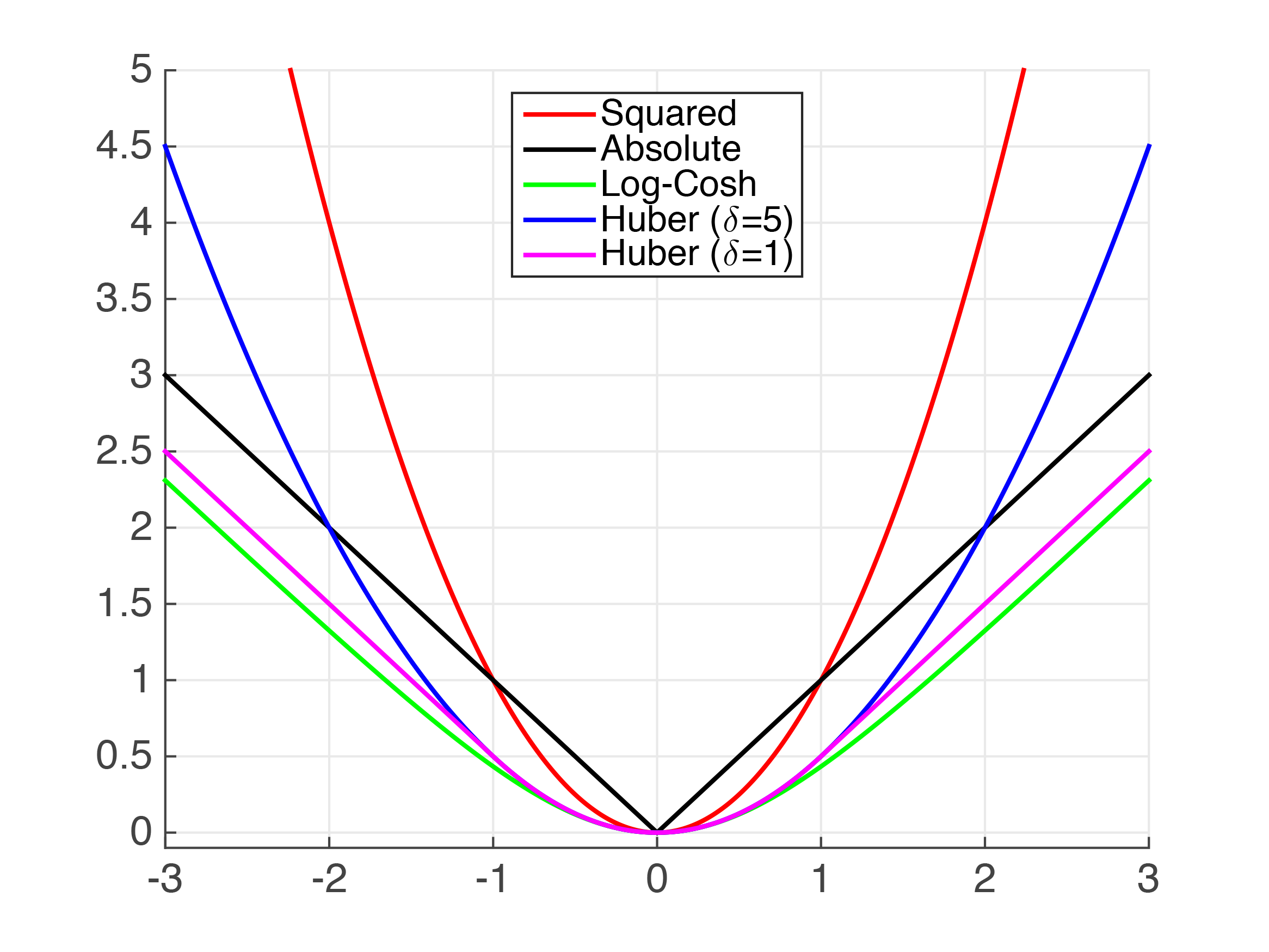
- Regression:Mean squared error is the most common loss function to optimize for unless there are a significant number of outliers. In this case, use mean absolute error orHuber loss.
- Classification: Cross-entropy will serve you well in most cases.
Batch Size
- Large batch sizes can be great because they can harness the power of GPUs to process more training instances per time. OpenAI has found larger batch sizes (of tens of thousands for image-classification and language modeling, and of millions in the case of RL agents) serve well for scaling and parallelizability.
- There’s a case to be made for smaller batch sizes, too, however. According to this paper by Masters and Luschi, the advantage gained from increased parallelism from running large batches is offset by the increased performance generalization and smaller memory footprint achieved by smaller batches. They show that increased batch sizes reduce the acceptable range of learning rates that provide stable convergence. Their takeaway is that smaller is, in-fact, better; and that the best performance is obtained by mini-batch sizes between 2 and 32.
- If you’re not operating at massive scales, I would recommend starting with lower batch sizes and slowly increasing the size and monitoring performance in your Weights and Biases dashboard to determine the best fit.
Number of epochs
- I’d recommend starting with a large number of epochs and use Early Stopping (see section 4. Vanishing + Exploding Gradients) to halt training when performance stops improving.
Scaling your features
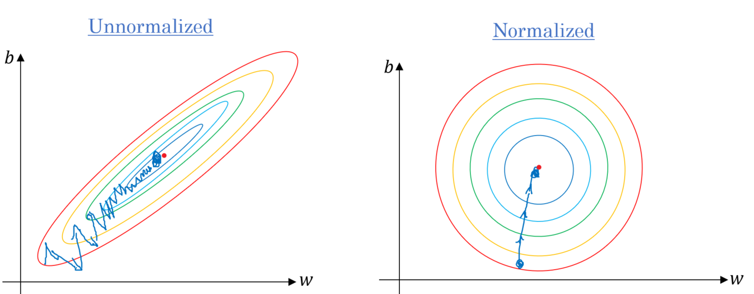
- A quick note: Make sure all your features have a similar scale before using them as inputs to your neural network. This ensures faster convergence. When your features have different scales (e.g., salaries in thousands and years of experience in tens), the cost function will look like the elongated bowl on the left. This means your optimization algorithm will take a long time to traverse the valley compared to using normalized features (on the right).
2. Learning Rate
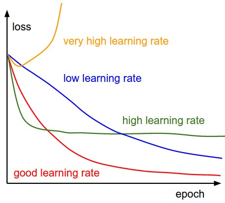
- Picking the learning rate is very important, and you want to make sure you get this right! Ideally, you want to re-tweak the learning rate when you tweak the other hyper-parameters of your network.
- To find the best learning rate, start with a very low value (10^-6) and slowly multiply it by a constant until it reaches a very high value (e.g., 10). Measure your model performance (vs. the log of your learning rate) in your Weights and Biases dashboard to determine which rate served you well for your problem. You can then retrain your model using this optimal learning rate.
- The best learning rate is usually half of the learning rate that causes the model to diverge. Feel free to set different values for learn_rate in the accompanying code and seeing how it affects model performance to develop your intuition around learning rates.
- I’d also recommend using the Learning Rate finder method proposed by Leslie Smith. It an excellent way to find a good learning rate for most gradient optimizers (most variants of SGD) and works with most network architectures.
- Also, see the section on learning rate scheduling below.
3. Momentum
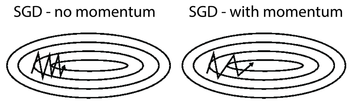
- Gradient Descent takes tiny, consistent steps towards the local minima and when the gradients are tiny it can take a lot of time to converge. Momentum, on the other hand, takes into account the previous gradients, and accelerates convergence by pushing over valleys faster and avoiding local minima.
- In general, you want your momentum value to be very close to one. 0.9 is a good place to start for smaller datasets, and you want to move progressively closer to one (0.999) the larger your dataset gets. (Setting nesterov=True lets momentum take into account the gradient of the cost function a few steps ahead of the current point, which makes it slightly more accurate and faster.)
4. Vanishing + Exploding Gradients
- Just like people, not all neural network layers learn at the same speed. So when the backprop algorithm propagates the error gradient from the output layer to the first layers, the gradients get smaller and smaller until they’re almost negligible when they reach the first layers. This means the weights of the first layers aren’t updated significantly at each step.
- This is the problem of vanishing gradients. (A similar problem of exploding gradients occurs when the gradients for certain layers get progressively larger, leading to massive weight updates for some layers as opposed to the others.)
- There are a few ways to counteract vanishing gradients. Let’s take a look at them now!
Activation functions
Hidden Layer Activation
In general, the performance from using different activation functions improves in this order (from lowest→highest performing): logistic → tanh → ReLU → Leaky ReLU → ELU → SELU.
ReLU is the most popular activation function and if you don’t want to tweak your activation function, ReLU is a great place to start. But, keep in mind ReLU is becoming increasingly less effective than ELU or GELU.
If you’re feeling more adventurous, you can try the following:
- to combat neural network overfitting: RReLU
- reduce latency at runtime: leaky ReLU
- for massive training sets: PReLU
- for fast inference times: leaky ReLU
- if your network doesn’t self-normalize: ELU
- for an overall robust activation function: SELU
As always, don’t be afraid to experiment with a few different activation functions, and turn to your Weights and Biases dashboard to help you pick the one that works best for you!
This is an excellent paper that dives deeper into the comparison of various activation functions for neural networks.
Output Layer Activation
Regression: Regression problems don’t require activation functions for their output neurons because we want the output to take on any value. In cases where we want out values to be bounded into a certain range, we can use tanh for -1→1 values and logistic function for 0→1 values. In cases where we’re only looking for positive output, we can use softplus activation.
Classification: Use the sigmoid activation function for binary classification to ensure the output is between 0 and 1. Use softmax for multi-class classification to ensure the output probabilities add up to 1.
Weight initialization method
- The right weight initialization method can speed up time-to-convergence considerably. The choice of your initialization method depends on your activation function. Some things to try:
- When using ReLU or leaky RELU, use He initialization
- When using SELU or ELU, use LeCun initialization
- When using softmax, logistic, or tanh, use Glorot initialization
- Most initialization methods come in uniform and normal distribution flavors.
BatchNorm
- BatchNorm simply learns the optimal means and scales of each layer’s inputs. It does so by zero-centering and normalizing its input vectors, then scaling and shifting them. It also acts like a regularizer, which means we don’t need dropout or L2 reg.
- Using BatchNorm lets us use larger learning rates (which result in faster convergence) and lead to huge improvements in most neural networks by reducing the vanishing gradients problem. The only downside is that it slightly increases training times because of the extra computations required at each layer.
Gradient Clipping
- A great way to reduce gradients from exploding, especially when training RNNs, is to simply clip them when they exceed a certain value. I’d recommend trying clipnorm instead of clipvalue, which allows you to keep the direction of your gradient vector consistent. Clipnorm contains any gradients who’s l2 norm is greater than a certain threshold.
- Try a few different threshold values to find one that works best for you.
Early Stopping
- Early Stopping lets you live it up by training a model with more hidden layers, hidden neurons and for more epochs than you need, and just stopping training when performance stops improving consecutively for n epochs. It also saves the best performing model for you. You can enable Early Stopping by setting up a callback when you fit your model and setting save_best_only=True.
5. Dropout
- Dropout is a fantastic regularization technique that gives you a massive performance boost (~2% for state-of-the-art models) for how simple the technique actually is. All dropout does is randomly turn off a percentage of neurons at each layer, at each training step. This makes the network more robust because it can’t rely on any particular set of input neurons for making predictions. The knowledge is distributed amongst the whole network. Around 2^n (where n is the number of neurons in the architecture) slightly-unique neural networks are generated during the training process and ensembled together to make predictions.
- A good dropout rate is between 0.1 to 0.5, 0.3 for RNNs, and 0.5 for CNNs. Use larger rates for bigger layers. Increasing the dropout rate decreases overfitting, and decreasing the rate is helpful to combat under-fitting.
- You want to experiment with different rates of dropout values in earlier layers of your network and check your Weights and Biases dashboard to pick the best performing one. You definitely don’t want to use dropout in the output layers.
- Read this paper before using Dropout in conjunction with BatchNorm.
- In this kernel, I used AlphaDropout, a flavor of the vanilla dropout that works well with SELU activation functions by preserving the input’s mean and standard deviations.
6. Optimizers
- Gradient Descent isn’t the only optimizer game in town! There are a few different ones to choose from. This post does a good job of describing some of the optimizers you can choose from.
- My general advice is to use Stochastic Gradient Descent if you care deeply about the quality of convergence and if time is not of the essence.
- If you care about time-to-convergence and a point close to optimal convergence will suffice, experiment with Adam, Nadam, RMSProp, and Adamax optimizers. Your Weights and Biases dashboard will guide you to the optimizer that works best for you!
- Adam/Nadam are usually good starting points and tend to be quite forgiving to bad learning rates and other non-optimal hyperparameters.
- According to Andrej Karpathy, “a well-tuned SGD will almost always slightly outperform Adam” in the case of ConvNets.
- In this kernel, I got the best performance from Nadam, which is just your regular Adam optimizer with the Nesterov trick, and thus converges faster than Adam.
7. Learning Rate Scheduling

- We talked about the importance of a good learning rate already — we don’t want it to be too high, lest the cost function dance around the optimum value and diverge. We also don’t want it to be too low because that means convergence will take a very long time.
- Babysitting the learning rate can be tough because both higher and lower learning rates have their advantages. The great news is that we don’t have to commit to one learning rate! With learning rate scheduling we can start with higher rates to move faster through gradient slopes, and slow it down when we reach a gradient valley in the hyper-parameter space, which requires taking smaller steps.
- There are many ways to schedule learning rates including decreasing the learning rate exponentially, or by using a step function, or tweaking it when the performance starts dropping or using 1cycle scheduling. In this kernel, I show you how to use the ReduceLROnPlateau callback to reduce the learning rate by a constant factor whenever the performance drops for n epochs.
- I would highly recommend also trying out 1cycle scheduling.
- Use a constant learning rate until you’ve trained all other hyper-parameters. And implement learning rate decay scheduling at the end.
- As with most things, I’d recommend running a few different experiments with different scheduling strategies and using your Weights and Biases dashboard to pick the one that leads to the best model.
A Few More Things
- Try EfficientNets to scale your network in an optimal way.
- Read this paper for an overview of some additional learning rates, batch sizes, momentum, and weight decay techniques.
- And this one on Stochastic Weight Averaging (SWA). It shows that better generalization can be achieved by averaging multiple points along the SGD’s trajectory, with a cyclical or constant learning rate.
- Read Andrej Karpathy’s excellent guide on getting the most juice out of your neural networks.
Results
We’ve explored a lot of different facets of neural networks in this post!
We’ve looked at how to set up a basic neural network (including choosing the number of hidden layers, hidden neurons, batch sizes, etc.)
We’ve learned about the role momentum and learning rates play in influencing model performance.
And finally, we’ve explored the problem of vanishing gradients and how to tackle it using non-saturating activation functions, BatchNorm, better weight initialization techniques and early stopping.
You can compare the accuracy and loss performances for the various techniques we tried in one single chart, by visiting your Weights and Biases dashboard.
Neural networks are powerful beasts that give you a lot of levers to tweak to get the best performance for the problems you’re trying to solve! The sheer size of customizations that they offer can be overwhelming to even seasoned practitioners. Tools like Weights and Biases are your best friends in navigating the land of the hyper-parameters, trying different experiments and picking the most powerful models.
I hope this guide will serve as a good starting point in your adventures. Good luck! I highly recommend forking this kernel and playing with the different building blocks to hone your intuition.
Bio: Lavanya is a machine learning engineer at Weights and Biases. She began working on AI 10 years ago when she founded ACM SIGAI at Purdue University as a sophomore. In a past life, she taught herself to code at age 10, and built her first startup at 14. She's driven by a deep desire to understand the universe around us better by using machine learning.
Related: