Beginner’s Guide to K-Nearest Neighbors in R: from Zero to Hero

This post presents a pipeline of building a KNN model in R with various measurement metrics.

By Leihua Ye, UC Santa Barbara

“If you live 5-min away from Bill Gates, I bet you are rich.”

Background

In the world of Machine Learning, I find the K-Nearest Neighbors (KNN) classifier makes the most intuitive sense and easily accessible to beginners even without introducing any math notations.

To decide the label of an observation, we look at its neighbors and assign the neighbors’ label to the observation of interest. Certainly, looking at one neighbor may create bias and inaccuracy, and the KNN method has a set of rules and procedures to determine the best number of neighbors, e.g., examining k>1 neighbors and adopt majority rule to decide the category.

Agor153

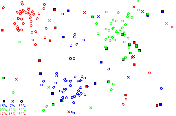
“To decide the label for new observations, we look at the closest neighbors.”

Measure of Distance

To choose the nearest neighbors, we have to define what distance is. For categorical data, there are Hamming Distance and Edit Distance. More information can be found here, as I won’t delve into the math in this post.

What is K-Fold Cross Validation?

In Machine Learning, Cross-Validation (CV) plays a crucial role in model selection and has a wide range of applications. In fact, CV has a rather straightforward design idea and also makes intuitive sense.

It can be briefly stated as follows:

divide the data into K equally distributed chunks/folds
choose 1 chunk/fold as a test set and the rest K-1 as a training set
develop an ML model based on the training set
compare predicted value VS true value on the test set only
apply the ML model to the test set and repeat K times using each chunk
add up the metrics score for the model and average over K folds

How to choose K?

As you probably noticed, the tricky part of CV is how to set the value for K. Let’s say the total sample size = n. Technically, we can set K to any value between 1 and n.

If k = n, we basically take 1 observation out as the training set and the rest n-1 cases as the test set. Then, repeat the process to the entire dataset. This is called “Leave-one-out cross-validation” (LOOCV).

Well, LOOCV requires a lot of computational power and may run forever if your dataset is big. Take a step back, there is no such thing as the best k value, and neither is it true that a higher k is a better k.

To choose the most appropriate k folds, we have to make a tradeoff between bias and variance. If k is small, we have a high bias but a low variance for estimating test error; if k is big, we have a low bias and a high variance.

Photo by Jon Tyson on Unsplash

“Hello Neighbor! Come On In.”

Implementation in R

1. Software Preparation

# install.packages(“ISLR”)
# install.packages(“ggplot2”) # install.packages(“plyr”)
# install.packages(“dplyr”) # install.packages(“class”)# Load libraries
library(ISLR) 
library(ggplot2) 
library(reshape2) 
library(plyr) 
library(dplyr) 
library(class)# load data and clean the dataset
banking=read.csv(“bank-additional-full.csv”,sep =”;”,header=T)##check for missing data and make sure no missing data
banking[!complete.cases(banking),]#re-code qualitative (factor) variables into numeric
banking$job= recode(banking$job, “‘admin.’=1;’blue-collar’=2;’entrepreneur’=3;’housemaid’=4;’management’=5;’retired’=6;’self-employed’=7;’services’=8;’student’=9;’technician’=10;’unemployed’=11;’unknown’=12”)#recode variable again
banking$marital = recode(banking$marital, “‘divorced’=1;’married’=2;’single’=3;’unknown’=4”)banking$education = recode(banking$education, “‘basic.4y’=1;’basic.6y’=2;’basic.9y’=3;’high.school’=4;’illiterate’=5;’professional.course’=6;’university.degree’=7;’unknown’=8”)banking$default = recode(banking$default, “‘no’=1;’yes’=2;’unknown’=3”)banking$housing = recode(banking$housing, “‘no’=1;’yes’=2;’unknown’=3”)banking$loan = recode(banking$loan, “‘no’=1;’yes’=2;’unknown’=3”)banking$contact = recode(banking$loan, “‘cellular’=1;’telephone’=2;”)banking$month = recode(banking$month, “‘mar’=1;’apr’=2;’may’=3;’jun’=4;’jul’=5;’aug’=6;’sep’=7;’oct’=8;’nov’=9;’dec’=10”)banking$day_of_week = recode(banking$day_of_week, “‘mon’=1;’tue’=2;’wed’=3;’thu’=4;’fri’=5;”)banking$poutcome = recode(banking$poutcome, “‘failure’=1;’nonexistent’=2;’success’=3;”)#remove variable “pdays”, b/c it has no variation
banking$pdays=NULL #remove variable “duration”, b/c itis collinear with the DV
banking$duration=NULL

After loading and cleaning the original dataset, it is a common practice to visually examine the distribution of our variables, checking for seasonality, patterns, outliers, etc.

#EDA of the DV
plot(banking$y,main="Plot 1: Distribution of Dependent Variable")

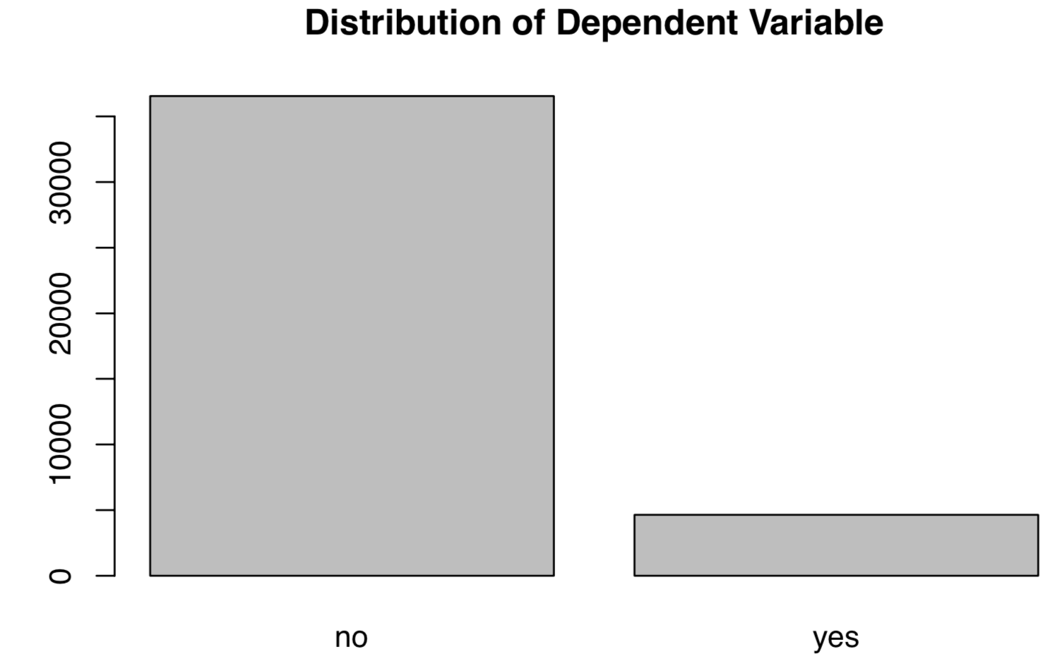
As can be seen, the Outcome Variables (Banking Service Subscription) are not equally distributed, with many more “No”s than “Yes”s.

This is unsurprisingly inconvenient for supervised learning when we try to classify future labels correctly. As expected, the rate of false positive would be high as a lot of minority cases would be classified as the majority label.

In fact, the unbalanced distribution may prefer a non-parametric ML classifier, as my other post (Rare Event Classification Using 5 Classifiers) shows KNN performs the best after comparing it to other ML methods. This may be caused by the underlying maths and statistical assumptions between parametric and non-parametric models.

2. Data Split

As mentioned above, we need to split the dataset into a training set and a test set and adopt k-fold cross-validation to pick the best ML model. A rule of thumb, we stick to the “80–20” division: we train ML models on 80% of the data and test it on the rest 20%. Slightly different for Time Series data, we change to 90% VS 10%.

#split the dataset into training and test sets randomly, but we need to set seed so as to generate the same value each time we run the codeset.seed(1)#create an index to split the data: 80% training and 20% test
index = round(nrow(banking)*0.2,digits=0)#sample randomly throughout the dataset and keep the total number equal to the value of index
test.indices = sample(1:nrow(banking), index)#80% training set
banking.train=banking[-test.indices,] #20% test set
banking.test=banking[test.indices,] #Select the training set except the DV
YTrain = banking.train$y
XTrain = banking.train %>% select(-y)# Select the test set except the DV
YTest = banking.test$y
XTest = banking.test %>% select(-y)

So far, we have finished data preparations and move on to model selection.

3. Train Models

Let’s create a new function (“calc_error_rate”) to record the misclassification rate. The function calculates the rate when the predicted label using the training model does not match with the actual outcome label. It measures classification accuracy.

#define an error rate function and apply it to obtain test/training errorscalc_error_rate <- function(predicted.value, true.value){
 return(mean(true.value!=predicted.value)) 
}

Then, we need another function, “do.chunk()”, to do k-fold Cross Validation. The function returns a data frame of the possible values of folds. The main purpose of this step is to select the best K value for KNN.

nfold = 10
set.seed(1)# cut() divides the range into several intervals
folds = seq.int(nrow(banking.train)) %>%
     cut(breaks = nfold, labels=FALSE) %>%  
     sampledo.chunk <- function(chunkid, folddef, Xdat, Ydat, k){ 
     train = (folddef!=chunkid)# training indexXtr = Xdat[train,] # training set by the indexYtr = Ydat[train] # true label in training setXvl = Xdat[!train,] # test setYvl = Ydat[!train] # true label in test setpredYtr = knn(train = Xtr, test = Xtr, cl = Ytr, k = k) # predict training labelspredYvl = knn(train = Xtr, test = Xvl, cl = Ytr, k = k) # predict test labelsdata.frame(fold =chunkid, # k folds 
train.error = calc_error_rate(predYtr, Ytr),#training error per fold 
 val.error = calc_error_rate(predYvl, Yvl)) # test error per fold
 }# set error.folds to save validation errors
error.folds=NULL# create a sequence of data with an interval of 10
kvec = c(1, seq(10, 50, length.out=5))set.seed(1)for (j in kvec){
 tmp = ldply(1:nfold, do.chunk, # apply do.function to each fold
 folddef=folds, Xdat=XTrain, Ydat=YTrain, k=j) # required arguments
 tmp$neighbors = j # track each value of neighbors
 error.folds = rbind(error.folds, tmp) # combine the results 
 }#melt() in the package reshape2 melts wide-format data into long-format data
errors = melt(error.folds, id.vars=c(“fold”,”neighbors”), value.name= “error”)

The upcoming step is to find the number of k that minimizes validation error

val.error.means = errors %>%
    #select all rows of validation errors
    filter(variable== “val.error” ) %>% 
    #group the selected data by neighbors
    group_by(neighbors, variable) %>%
    #cacluate CV error for each k
    summarise_each(funs(mean), error) %>%
    #remove existing grouping
    ungroup() %>% 
    filter(error==min(error))#the best number of neighbors
numneighbor = max(val.error.means$neighbors)
numneighbor## [20]

Therefore, the best number of neighbors is 20 after using 10-fold cross-validation.

Nick Youngson

4. Some Model Metrics

#training error
set.seed(20)
pred.YTtrain = knn(train=XTrain, test=XTrain, cl=YTrain, k=20)knn_traing_error <- calc_error_rate(predicted.value=pred.YTtrain, true.value=YTrain)
knn_traing_error[1] 0.101214

The training error is 0.10.

#test error
set.seed(20)
pred.YTest = knn(train=XTrain, test=XTest, cl=YTrain, k=20)knn_test_error <- calc_error_rate(predicted.value=pred.YTest, true.value=YTest)
knn_test_error[1] 0.1100995

The test error is 0.11.

#confusion matrixconf.matrix = table(predicted=pred.YTest, true=YTest)

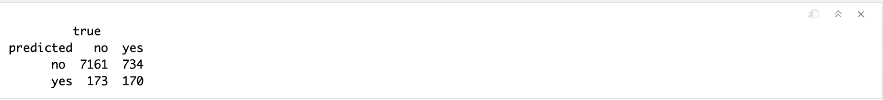
Based on the above confusion matrix, we can calculate the following values and prepare for plotting the ROC curve.

Accuracy = (TP +TN)/(TP+FP+FN+TN)

TPR/Recall/Sensitivity = TP/(TP+FN)

Precision = TP/(TP+FP)

Specificity = TN/(TN+FP)

FPR = 1 — Specificity = FP/(TN+FP)

F1 Score = 2*TP/(2*TP+FP+FN) = Precision*Recall /(Precision +Recall)

# Test accuracy ratesum(diag(conf.matrix)/sum(conf.matrix))[1] 0.8899005# Test error rate1 - sum(drag(conf.matrix)/sum(conf.matrix))[1] 0.1100995

As you may notice, test accuracy rate + test error rate = 1, and I’m providing multiple ways of calculating each value.

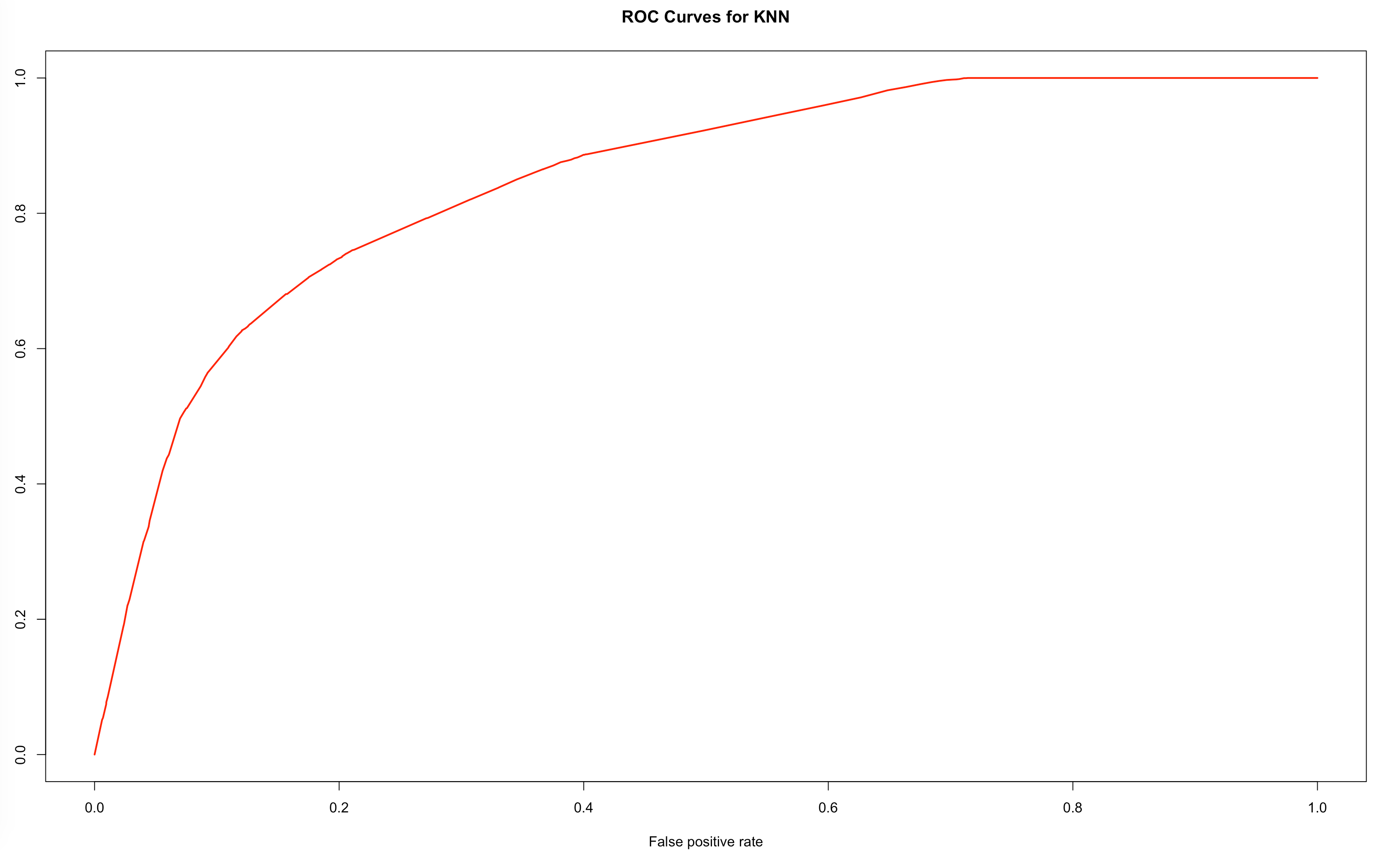
# ROC and AUC
knn_model = knn(train=XTrain, test=XTrain, cl=YTrain, k=20,prob=TRUE)prob <- attr(knn_model, “prob”)prob <- 2*ifelse(knn_model == “-1”, prob,1-prob) — 1pred_knn <- prediction(prob, YTrain)performance_knn <- performance(pred_knn, “tpr”, “fpr”)# AUCauc_knn <- performance(pred_knn,”auc”)@y.valuesauc_knn[1] 0.8470583plot(performance_knn,col=2,lwd=2,main=”ROC Curves for KNN”)

In conclusion, we have learned what KNN is and built a pipeline of building a KNN model in R. More importantly, we have learned the underlying idea behind K-Fold Cross-validation and how to cross-validate in R.

Enjoy reading this one? If so, please check my other posts on Machine Learning and programming.

Supervised ML:

A Big Challenge: How to Predict Rare Events using 5 Machine Learning Methods
Which ML method works best when the outcome variable is highly imbalanced? What are the tradeoffs?

Machine Learning 101: Predicting Drug Use Using Logistic Regression In R
Basics, link functions, and plots

Machine Learning 102: Logistic Regression With Polynomial Features
How to classify when there are nonlinear components

Unsupervised ML:

Unsupervised Machine Learning: Using PCA and Hierarchical Clustering To Analyze Genes and Leukemia
A real-life application of unsupervised learning

Image Compression In 10 Lines of R Code
An innovative way of using PCA in dimension reduction

Bio: Leihua Ye (@leihua_ye)is a Ph.D. Candidate at the UC, Santa Barbara. He has 5+ years of research and professional experience in Quantitative UX Research, Experimentation & Causal Inference, Machine Learning, and Data Science.

Original. Reposted with permission.

Related: