Introduction to k-Nearest Neighbors

comments

By Devin Soni, Computer Science Student

The k-Nearest-Neighbors (kNN) method of classification is one of the simplest methods in machine learning, and is a great way to introduce yourself to machine learning and classification in general. At its most basic level, it is essentially classification by finding the most similar data points in the training data, and making an educated guess based on their classifications. Although very simple to understand and implement, this method has seen wide application in many domains, such as in recommendation systems, semantic searching, and anomaly detection.

As we would need to in any machine learning problem, we must first find a way to represent data points as feature vectors. A feature vector is our mathematical representation of data, and since the desired characteristics of our data may not be inherently numerical, preprocessing and feature-engineering may be required in order to create these vectors. Given data with N unique features, the feature vector would be a vector of length N, where entry I of the vector represents that data point’s value for feature I. Each feature vector can thus be thought of as a point in R^N.

Now, unlike most other methods of classification, kNN falls under lazy learning, which means that there is no explicit training phase before classification. Instead, any attempts to generalize or abstract the data is made upon classification. While this does mean that we can immediately begin classifying once we have our data, there are some inherent problems with this type of algorithm. We must be able to keep the entire training set in memory unless we apply some type of reduction to the data-set, and performing classifications can be computationally expensive as the algorithm parse through all data points for each classification. For these reasons, kNN tends to work best on smaller data-sets that do not have many features.

Once we have formed our training data-set, which is represented as an M x N matrix where M is the number of data points and N is the number of features, we can now begin classifying. The gist of the kNN method is, for each classification query, to:

1. Compute a distance value between the item to be classified and every item in the training data-set

2. Pick the k closest data points (the items with the k lowest distances)

3. Conduct a “majority vote” among those data points — the dominating classification in that pool is decided as the final classification

There are two important decisions that must be made before making classifications. One is the value of k that will be used; this can either be decided arbitrarily, or you can try cross-validation to find an optimal value. The next, and the most complex, is the distance metric that will be used.

There are many different ways to compute distance, as it is a fairly ambiguous notion, and the proper metric to use is always going to be determined by the data-set and the classification task. Two popular ones, however, are Euclidean distance and Cosine similarity.

Euclidean distance is probably the one that you are most familiar with; it is essentially the magnitude of the vector obtained by subtracting the training data point from the point to be classified.

General formula for Euclidean distance

Another common metric is Cosine similarity. Rather than calculating a magnitude, Cosine similarity instead uses the difference in direction between two vectors.

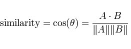
General formula for Cosine similarity

Choosing a metric can often be tricky, and it may be best to just use cross-validation to decide, unless you have some prior insight that clearly leads to using one over the other. For example, for something like word vectors, you may want to use Cosine similarity because the direction of a word is more meaningful than the sizes of the component values. Generally, both of these methods will run in roughly the same time, and will suffer from highly-dimensional data.

After doing all of the above and deciding on a metric, the result of the kNN algorithm is a decision boundary that partitions R^N into sections. Each section (colored distinctly below) represents a class in the classification problem. The boundaries need not be formed with actual training examples — they are instead calculated using the distance metric and the available training points. By taking R^N in (small) chunks, we can calculate the most likely class for a hypothetical data-point in that region, and we thus color that chunk as being in the region for that class.

This information is all that is needed to begin implementing the algorithm, and doing so should be relatively simple. There are, of course, many ways to improve upon this base algorithm. Common modifications include weighting, and specific preprocessing to reduce computation and reduce noise, such as various algorithms for feature extraction and dimension reduction. Additionally, the kNN method has also been used, although less-commonly, for regression tasks, and operates in a manner very similar to that of the classifier through averaging.

 
Bio: Devin Soni is a computer science student interested in machine learning and data science. He will be a software engineering intern at Airbnb in 2018. He can be reached via LinkedIn.

Original. Reposted with permission.

Related:

• Introduction to Markov Chains
• A Tour of The Top 10 Algorithms for Machine Learning Newbies
• K-Nearest Neighbors – the Laziest Machine Learning Technique