Visualizing Decision Trees with Python (Scikit-learn, Graphviz, Matplotlib)
Learn about how to visualize decision trees using matplotlib and Graphviz.
By Michael Galarnyk, Data Scientist
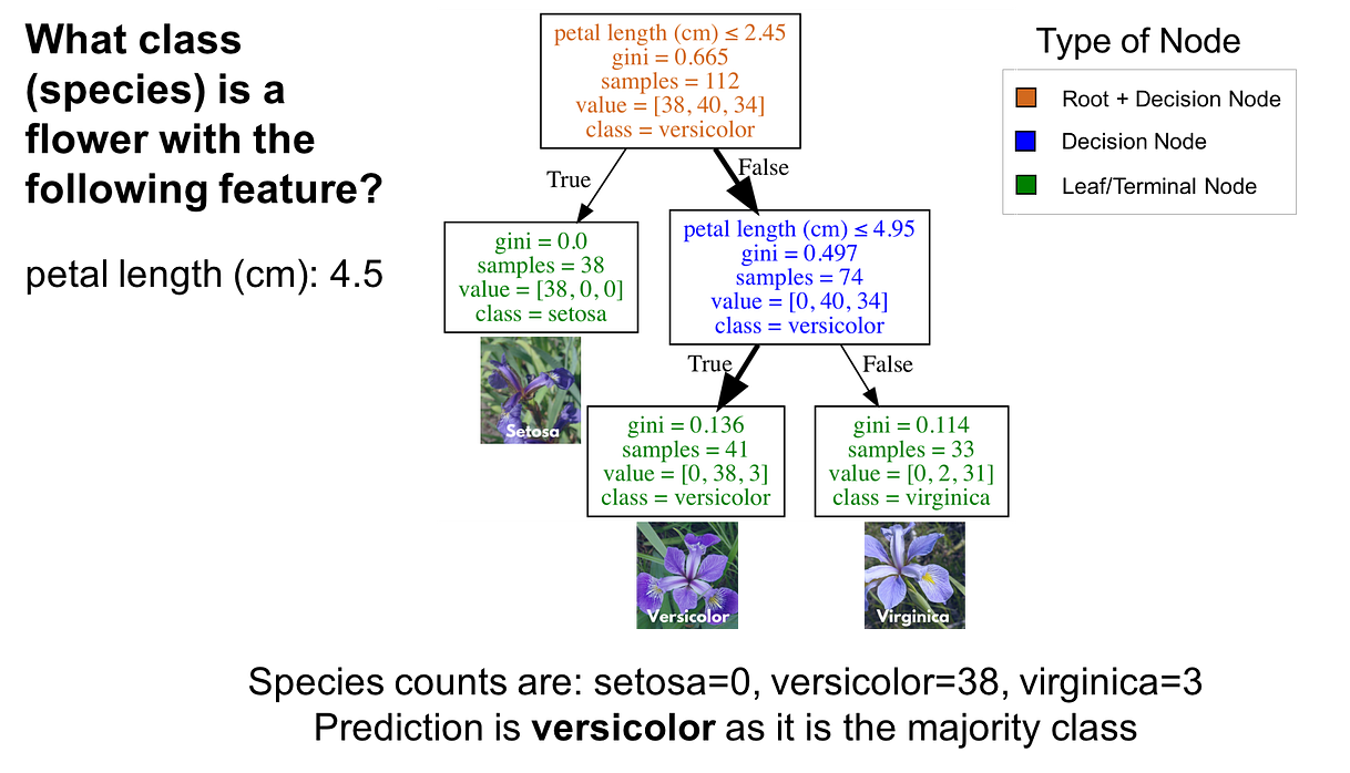
Decision trees are a popular supervised learning method for a variety of reasons. Benefits of decision trees include that they can be used for both regression and classification, they don’t require feature scaling, and they are relatively easy to interpret as you can visualize decision trees. This is not only a powerful way to understand your model, but also to communicate how your model works. Consequently, it would help to know how to make a visualization based on your model.
This tutorial covers:
- How to Fit a Decision Tree Model using Scikit-Learn
- How to Visualize Decision Trees using Matplotlib
- How to Visualize Decision Trees using Graphviz (what is Graphviz, how to install it on Mac and Windows, and how to use it to visualize decision trees)
- How to Visualize Individual Decision Trees from Bagged Trees or Random Forests®
As always, the code used in this tutorial is available on my GitHub. With that, let’s get started!
How to Fit a Decision Tree Model using Scikit-Learn
In order to visualize decision trees, we need first need to fit a decision tree model using scikit-learn. If this section is not clear, I encourage you to read my Understanding Decision Trees for Classification (Python) tutorial as I go into a lot of detail on how decision trees work and how to use them.
Import Libraries
The following import statements are what we will use for this section of the tutorial.
import matplotlib.pyplot as plt
from sklearn.datasets import load_iris
from sklearn.datasets import load_breast_cancer
from sklearn.tree import DecisionTreeClassifier
from sklearn.ensemble import RandomForestClassifier
from sklearn.model_selection import train_test_split
import pandas as pd
import numpy as np
from sklearn import tree
Load the Dataset
The Iris dataset is one of datasets scikit-learn comes with that do not require the downloading of any file from some external website. The code below loads the iris dataset.
import pandas as pd
from sklearn.datasets import load_irisdata = load_iris()
df = pd.DataFrame(data.data, columns=data.feature_names)
df['target'] = data.target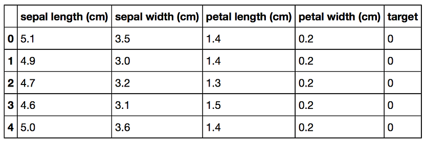
Splitting Data into Training and Test Sets
The code below puts 75% of the data into a training set and 25% of the data into a test set.
X_train, X_test, Y_train, Y_test = train_test_split(df[data.feature_names], df['target'], random_state=0)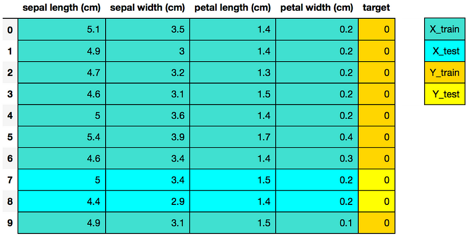
Scikit-learn 4-Step Modeling Pattern
# Step 1: Import the model you want to use
# This was already imported earlier in the notebook so commenting out
#from sklearn.tree import DecisionTreeClassifier# Step 2: Make an instance of the Model
clf = DecisionTreeClassifier(max_depth = 2,
                             random_state = 0)# Step 3: Train the model on the data
clf.fit(X_train, Y_train)# Step 4: Predict labels of unseen (test) data
# Not doing this step in the tutorial
# clf.predict(X_test)
How to Visualize Decision Trees using Matplotlib
As of scikit-learn version 21.0 (roughly May 2019), Decision Trees can now be plotted with matplotlib using scikit-learn’s tree.plot_tree without relying on the dot library which is a hard-to-install dependency which we will cover later on in the blog post.
The code below plots a decision tree using scikit-learn.
tree.plot_tree(clf);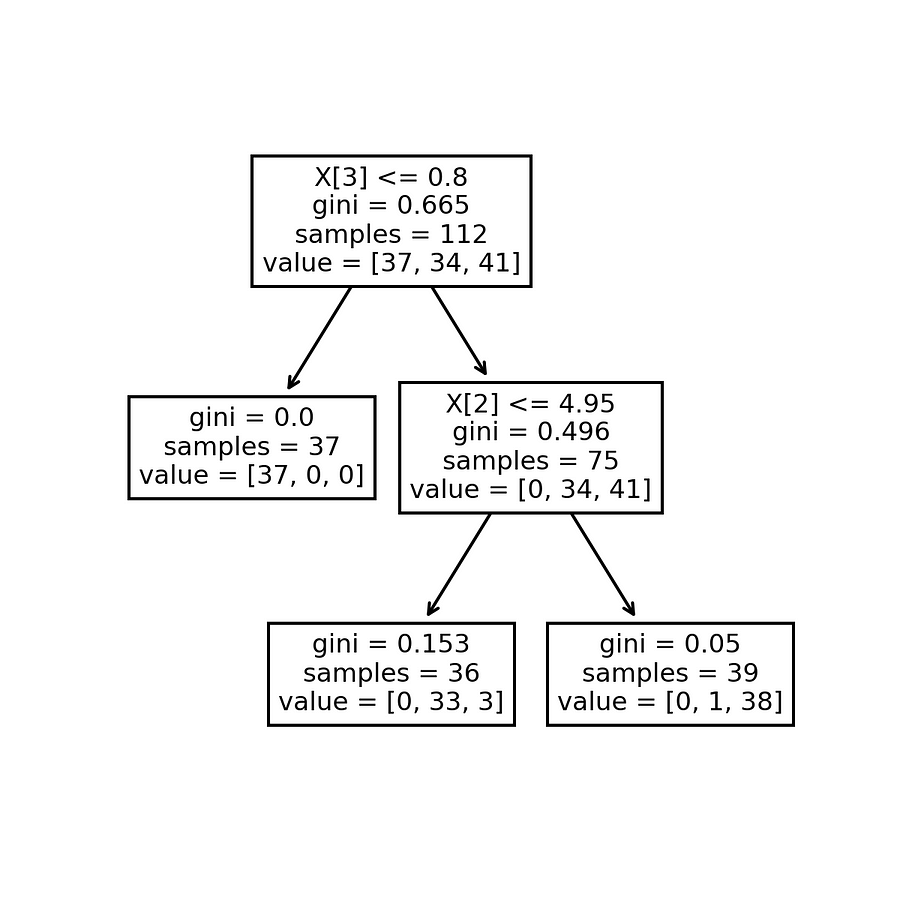
In addition to adding the code to allow you to save your image, the code below tries to make the decision tree more interpretable by adding in feature and class names (as well as setting filled = True).
fn=['sepal length (cm)','sepal width (cm)','petal length (cm)','petal width (cm)']
cn=['setosa', 'versicolor', 'virginica']fig, axes = plt.subplots(nrows = 1,ncols = 1,figsize = (4,4), dpi=300)tree.plot_tree(clf,
               feature_names = fn,
               class_names=cn,
               filled = True);fig.savefig('imagename.png')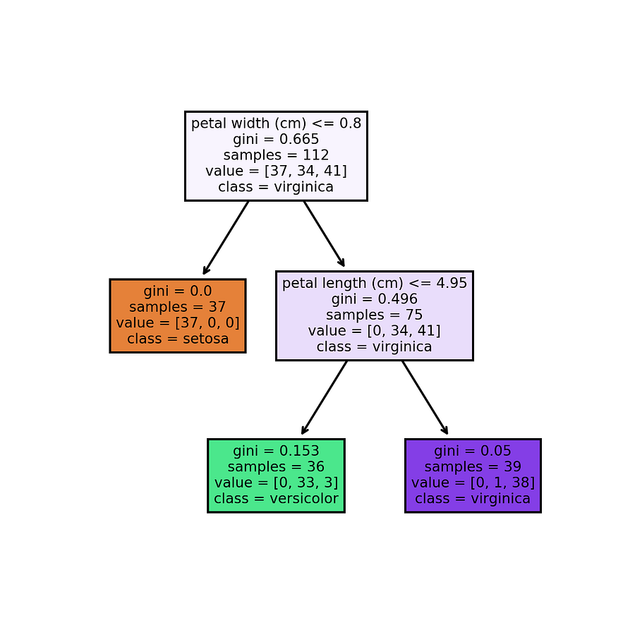
How to Visualize Decision Trees using Graphviz
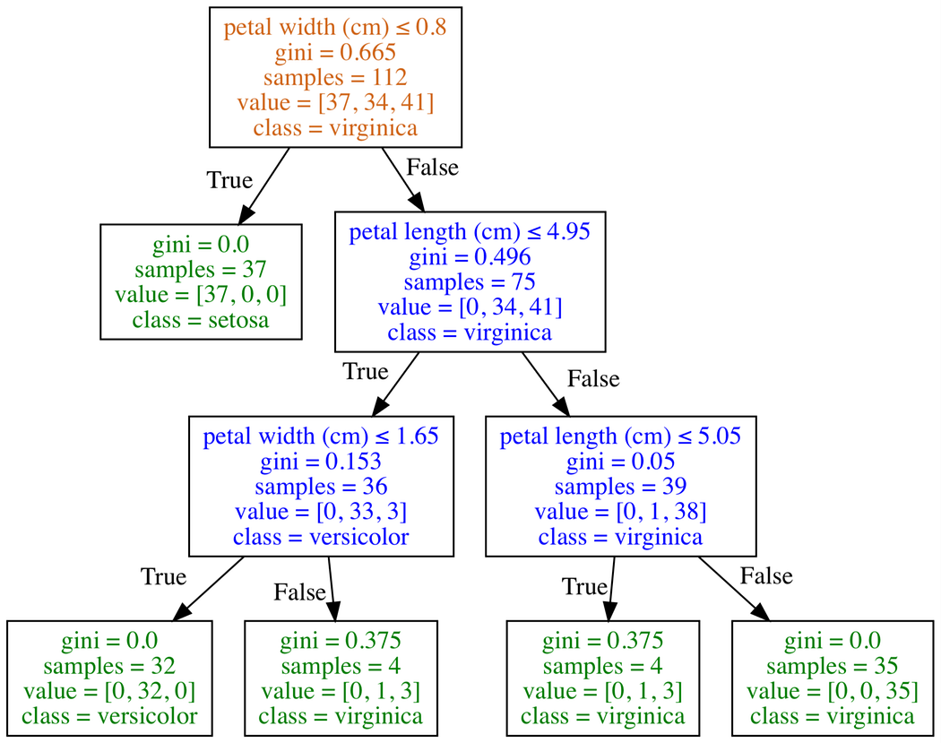
Graphviz is open source graph visualization software. Graph visualization is a way of representing structural information as diagrams of abstract graphs and networks. In data science, one use of Graphviz is to visualize decision trees. I should note that the reason why I am going over Graphviz after covering Matplotlib is that getting this to work can be difficult. The first part of this process involves creating a dot file. A dot file is a Graphviz representation of a decision tree. The problem is that using Graphviz to convert the dot file into an image file (png, jpg, etc) can be difficult. There are a couple ways to do this including: installing python-graphviz though Anaconda, installing Graphviz through Homebrew (Mac), installing Graphviz executables from the official site (Windows), and using an online converter on the contents of your dot file to convert it into an image.
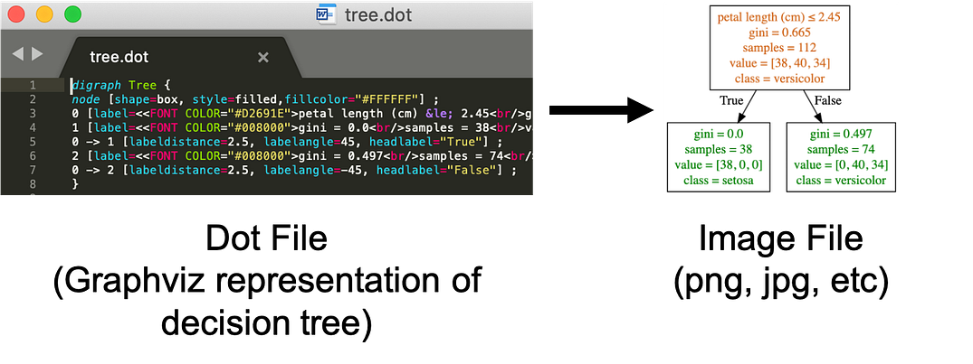
Export your model to a dot file
The code below code will work on any operating system as python generates the dot file and exports it as a file named tree.dot.
tree.export_graphviz(clf,
                     out_file="tree.dot",
                     feature_names = fn,
                     class_names=cn,
                     filled = True)
Installing and Using Graphviz
Converting the dot file into an image file (png, jpg, etc) typically requires the installation of Graphviz which depends on your operating system and a host of other things. The goal of this section is to help people try and solve the common issue of getting the following error. dot: command not found.
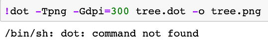
dot: command not found
How to Install and Use on Mac through Anaconda
To be able to install Graphviz on your Mac through this method, you first need to have Anaconda installed (If you don’t have Anaconda installed, you can learn how to install it here).
Open a terminal. You can do this by clicking on the Spotlight magnifying glass at the top right of the screen, type terminal and then click on the Terminal icon.

Type the command below to install Graphviz.
conda install python-graphvizAfter that, you should be able to use the dot command below to convert the dot file into a png file.
dot -Tpng tree.dot -o tree.pngHow to Install and Use on Mac through Homebrew
If you don’t have Anaconda or just want another way of installing Graphviz on your Mac, you can use Homebrew. I previously wrote an article on how to install Homebrew and use it to convert a dot file into an image file here (see the Homebrew to Help Visualize Decision Trees section of the tutorial).
How to Install and Use on Windows through Anaconda
This is the method I prefer on Windows. To be able to install Graphviz on your Windows through this method, you first need to have Anaconda installed (If you don’t have Anaconda installed, you can learn how to install it here).
Open a terminal/command prompt and enter the command below to install Graphviz.
conda install python-graphvizAfter that, you should be able to use the dot command below to convert the dot file into a png file.
dot -Tpng tree.dot -o tree.png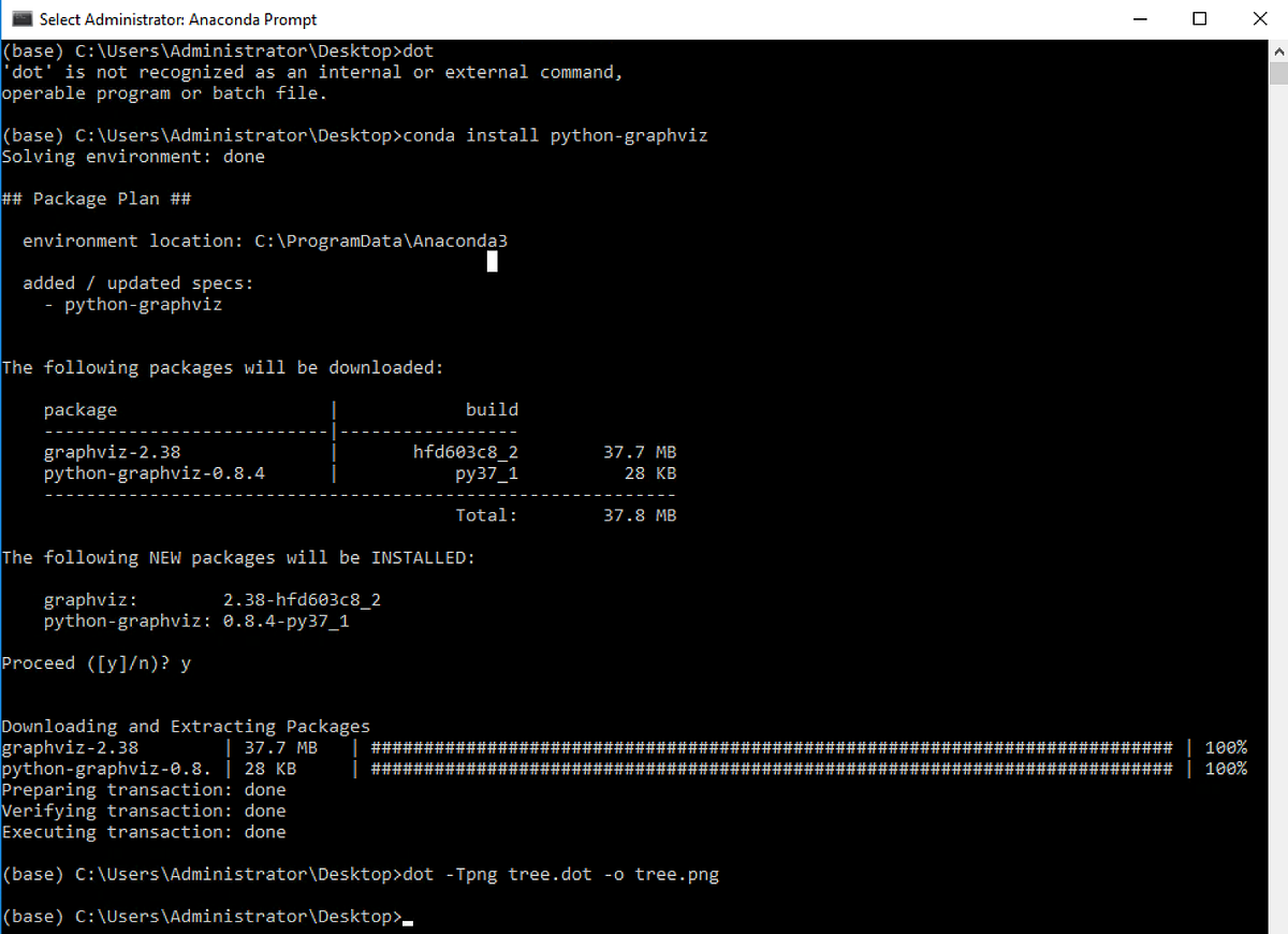
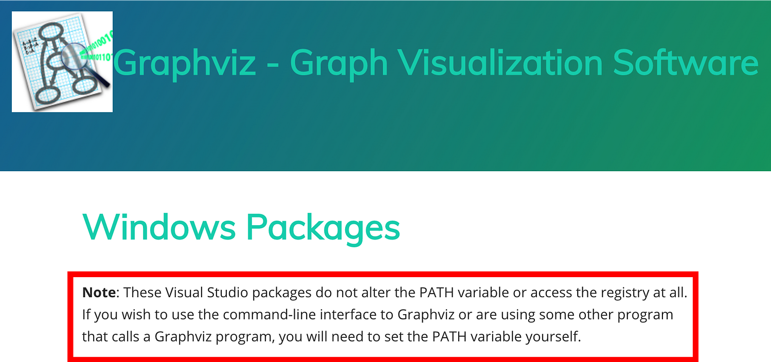
How to Install and Use on Windows through Graphviz Executable
If you don’t have Anaconda or just want another way of installing Graphviz on your Windows, you can use the following link to download and install it.
How to Use an Online Converter to Visualize your Decision Trees
If all else fails or you simply don’t want to install anything, you can use an online converter.
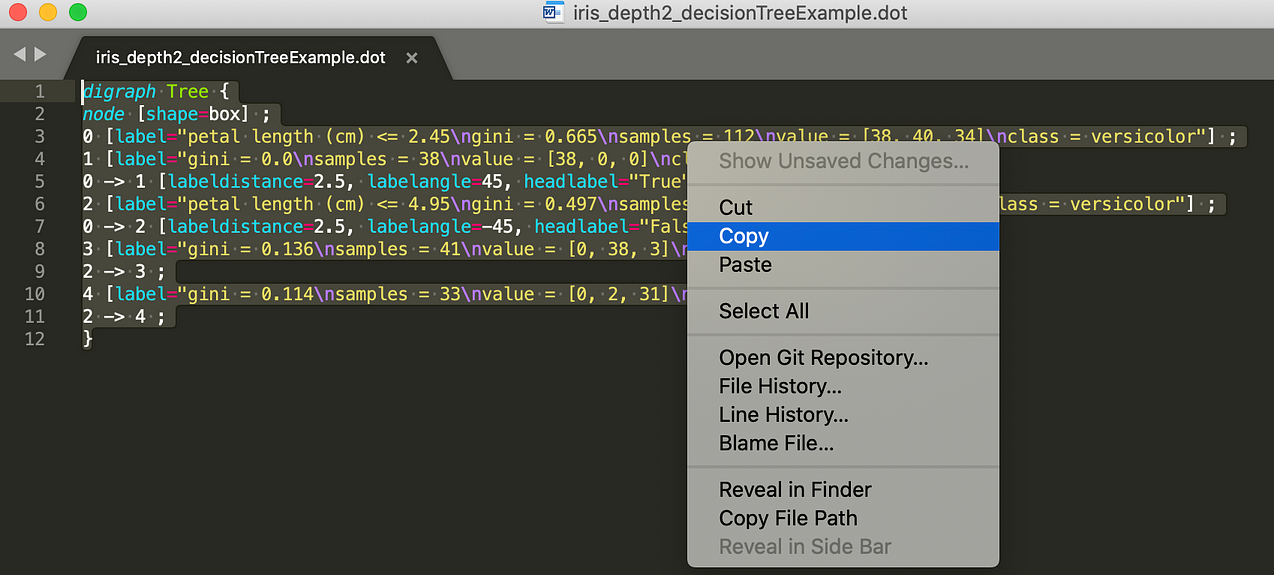
In the image below, I opened the file with Sublime Text (though there are many different programs that can open/read a dot file) and copied the content of the file.
In the image below, I pasted the content from the dot file onto the left side of the online converter. You can then choose what format you want and then save the image on the right side of the screen.
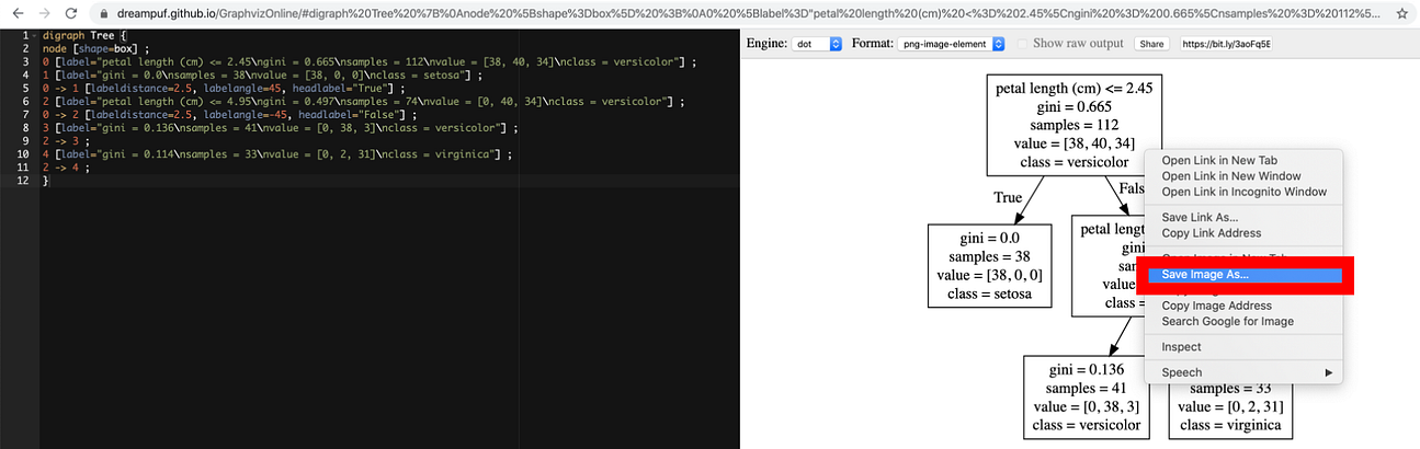
Keep in mind that there are other online converters that can help accomplish the same task.
How to Visualize Individual Decision Trees from Bagged Trees or Random Forests®
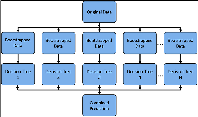
A weakness of decision trees is that they don’t tend to have the best predictive accuracy. This is partially because of high variance, meaning that different splits in the training data can lead to very different trees.
The image above could be a diagram for Bagged Trees or the random forest algorithm models which are ensemble methods. This means using multiple learning algorithms to obtain a better predictive performance than could be obtained from any of the constituent learning algorithms alone. In this case, many trees protect each other from their individual errors. How exactly Bagged Trees and the random forest algorithm models work is a subject for another blog, but what is important to note is that for each both models we grow N trees where N is the number of decision trees a user specifies. Consequently after you fit a model, it would be nice to look at the individual decision trees that make up your model.
Fit a Random Forest® Model using Scikit-Learn
In order to visualize individual decision trees, we need first need to fit a Bagged Trees or Random Forest® model using scikit-learn (the code below fits the random forest algorithm model).
# Load the Breast Cancer (Diagnostic) Dataset
data = load_breast_cancer()
df = pd.DataFrame(data.data, columns=data.feature_names)
df['target'] = data.target# Arrange Data into Features Matrix and Target Vector
X = df.loc[:, df.columns != 'target']
y = df.loc[:, 'target'].values# Split the data into training and testing sets
X_train, X_test, Y_train, Y_test = train_test_split(X, y, random_state=0)# Random Forests in `scikit-learn` (with N = 100)
rf = RandomForestClassifier(n_estimators=100,
                            random_state=0)
rf.fit(X_train, Y_train)
Visualizing your Estimators
You can now view all the individual trees from the fitted model. In this section, I will visualize all the decision trees using matplotlib.
rf.estimators_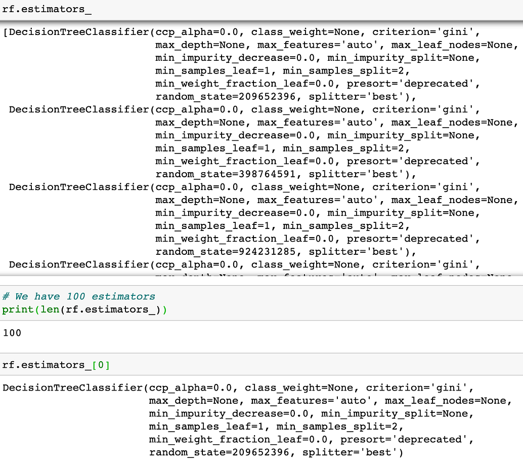
You can now visualize individual trees. The code below visualizes the first decision tree.
fn=data.feature_names
cn=data.target_names
fig, axes = plt.subplots(nrows = 1,ncols = 1,figsize = (4,4), dpi=800)
tree.plot_tree(rf.estimators_[0],
               feature_names = fn,
               class_names=cn,
               filled = True);
fig.savefig('rf_individualtree.png')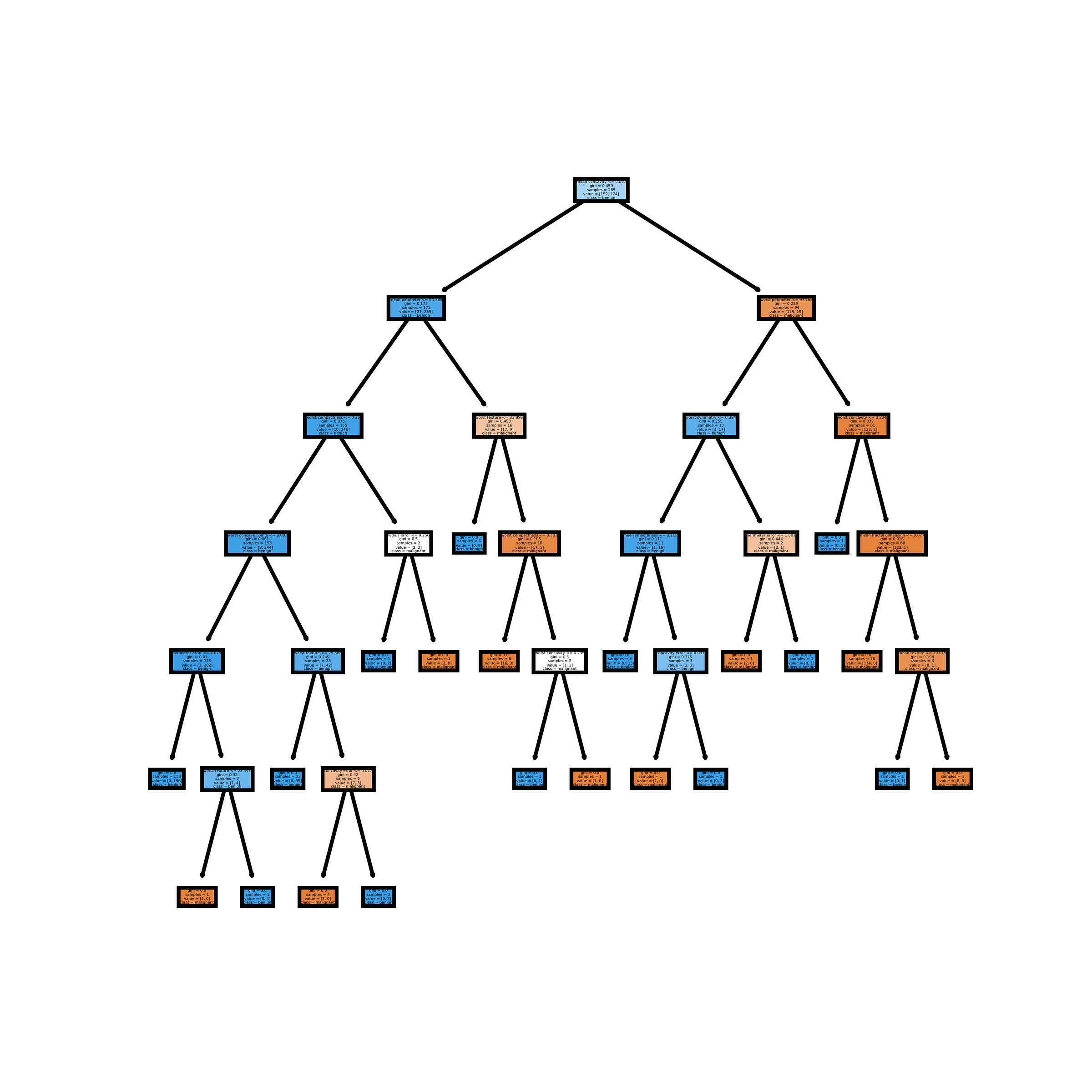
You can try to use matplotlib subplots to visualize as many of the trees as you like. The code below visualizes the first 5 decision trees. I personally don’t prefer this method as it is even harder to read.
# This may not the best way to view each estimator as it is smallfn=data.feature_names
cn=data.target_names
fig, axes = plt.subplots(nrows = 1,ncols = 5,figsize = (10,2), dpi=3000)for index in range(0, 5):
    tree.plot_tree(rf.estimators_[index],
                   feature_names = fn,
                   class_names=cn,
                   filled = True,
                   ax = axes[index]);

    axes[index].set_title('Estimator: ' + str(index), fontsize = 11)fig.savefig('rf_5trees.png')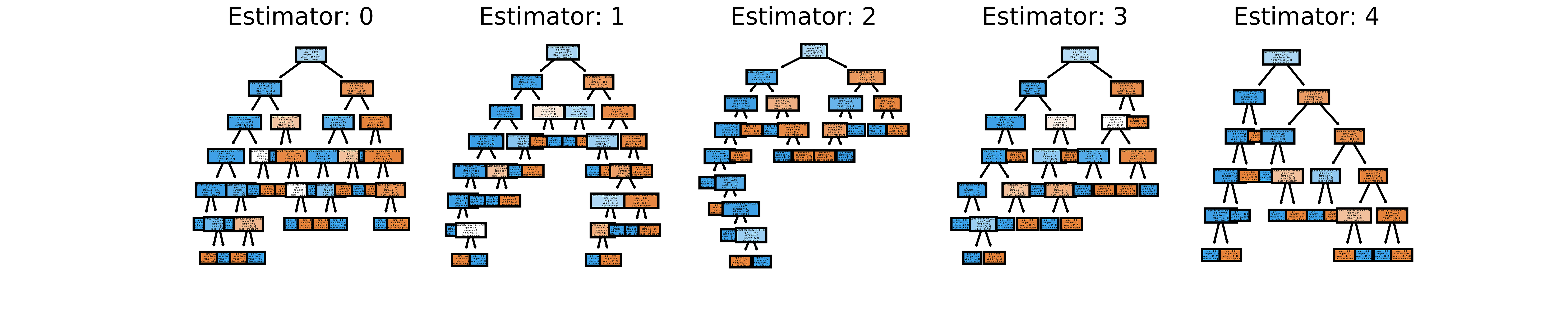
Create Images for each of the Decision Trees (estimators)
Keep in mind that if for some reason you want images for all your estimators (decision trees), you can do so using the code on my GitHub. If you just want to see each of the 100 estimators for the random forest algorithm model fit in this tutorial without running the code, you can look at the video below.
Concluding Remarks
This tutorial covered how to visualize decision trees using Graphviz and Matplotlib. Note that the way to visualize decision trees using Matplotlib is a newer method so it might change or be improved upon in the future. Graphviz is currently more flexible as you can always modify your dot files to make them more visually appealing like I did using the dot language or even just alter the orientation of your decision tree. One thing we didn’t cover was how to use dtreeviz which is another library that can visualize decision trees. There is an excellent post on it here.
If you have any questions or thoughts on the tutorial, feel free to reach out in the comments below or through Twitter. If you want to learn more about how to utilize Pandas, Matplotlib, or Seaborn libraries, please consider taking my Python for Data Visualization LinkedIn Learning course.
RANDOM FORESTS and RANDOMFORESTS are registered marks of Minitab, LLC.
Bio: Michael Galarnyk is a Data Scientist and Corporate Trainer. He currently works at Scripps Translational Research Institute. You can find him on Twitter (https://twitter.com/GalarnykMichael), Medium (https://medium.com/@GalarnykMichael), and GitHub (https://github.com/mGalarnyk).
Original. Reposted with permission.
Related:
- Understanding Decision Trees for Classification in Python
- Decision Tree Algorithm, Explained
- Decision Tree Intuition: From Concept to Application