Decision Tree Intuition: From Concept to Application

A decision tree is one of the popular and powerful machine learning algorithms that I have learned. It is a non-parametric supervised learning method that can be used for both classification and regression tasks. The goal is to create a model that predicts the value of a target variable by learning simple decision rules inferred from the data features. For a classification model, the target values are discrete in nature, whereas, for a regression model, the target values are represented by continuous values. Unlike the black box type of algorithms such as Neural Network, Decision Trees are comparably easier to understand because it shares internal decision-making logic (you will find details in the following session).

Despite the fact that many data scientists believe it’s an old method and they may have some doubts of its accuracy due to an overfitting problem, the more recent tree-based models, for example, Random forest (bagging method), gradient boosting (boosting method) and XGBoost (boosting method) are built on the top of decision tree algorithm. Therefore, the concepts and algorithms behind Decision Trees are strongly worth understanding!

There are 4 popular types of decision tree algorithms: ID3, CART (Classification and Regression Trees), Chi-Square, and Reduction in Variance.

In this blog, I will only focus on the classification trees and the explanations of ID3 and CART.

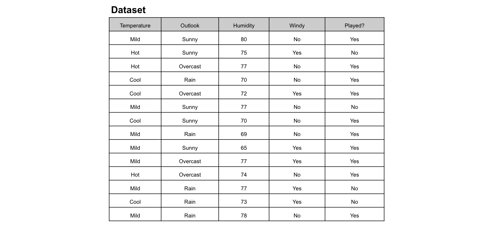
Imagine you play tennis every Sunday and you invite your best friend, Clare to come with you every time. Clare sometimes comes to join but sometimes not. For her, it depends on a number of factors, for example, weather, temperature, humidity, and wind. I would like to use the dataset below to predict whether or not Clare will join me to play tennis. An intuitive way to do this is through a Decision Tree.

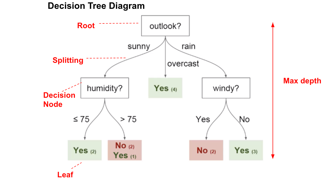
In this Decision Tree diagram, we have:

1. Root Node:The first split which decides the entire population or sample data should further get divided into two or more homogeneous sets. In our case, the Outlook node.
2. Splitting:It is a process of dividing a node into two or more sub-nodes.
3. Decision Node:This node decides whether/when a sub-node splits into further sub-nodes or not. Here we have, Outlook node, Humidity node, and Windy node.
4. Leaf:Terminal Node that predicts the outcome (categorical or continuous value). The coloured nodes, i.e., Yes and No nodes, are the leaves.

Question: Base on which attribute (feature) to split? What is the best split?

Answer: Use the attribute with the highest Information Gain or Gini Gain

ID3 (Iterative Dichotomiser)

ID3 decision tree algorithm uses Information Gain to decide the splitting points. In order to measure how much information we gain, we can use entropy to calculate the homogeneity of a sample.

Question: What is “Entropy”? and What is its function?

Answer: It is a measure of the amount of uncertainty in a data set. Entropy controls how a Decision Tree decides to split the data. It actually affects how a Decision Tree draws its boundaries.

The equation of Entropy:

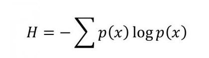
The logarithm of the probability distribution is useful as a measure of entropy.

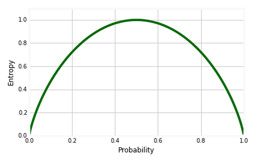
Entropy vs. Probability.

Definition: Entropy in Decision Tree stands for homogeneity.

If the sample is completely homogeneous, the entropy is 0 (prob= 0 or 1), and if the sample is evenly distributed across classes, it has an entropy of 1 (prob =0.5).

The next step is to make splits that minimize entropy. We use information gain to determine the best split.

Let me show you how to calculate the information gain step by step in the case of playing tennis. Here I will only show you how to calculate the Information Gain and Entropy of Outlook.

Step 1: Calculate the Entropy of one attribute — Prediction: Clare Will Play Tennis/ Clare Will Not Play Tennis

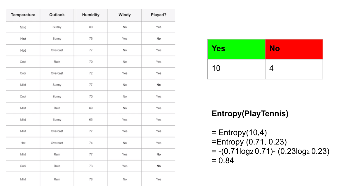
For this illustration, I will use this contingency table to calculate the entropy of our target variable: Played? (Yes/No). There are 14 observations (10 “Yes” and 4 “No”). The probability (p) of ‘Yes’ is 0.71428(10/14), and the probability of ‘No’ is 0.28571 (4/14). You can then calculate the entropy of our target variable using the equation above.

Step 2: Calculate the Entropy for each feature using the contingency table

To illustrate, I use Outlook as an example to explain how to calculate its Entropy. There are a total of 14 observations. Summing across the rows we can see there are 5 of them belong to Sunny, 4 belong to Overcast, and 5 belong to Rainy. Therefore, we can find the probability of Sunny, Overcast, and Rainy and then calculate their entropy one by one using the above equation. The calculation steps are shown below.

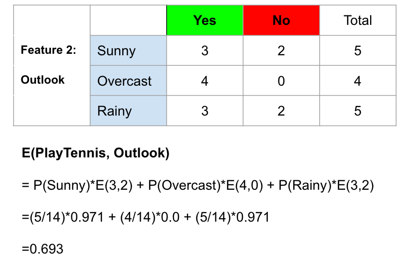
An example of calculating the entropy of feature 2 (Outlook).

Definition: Information Gain is the decrease or increase in Entropy value when the node is split.

The equation of Information Gain:

Information Gain from X on Y.

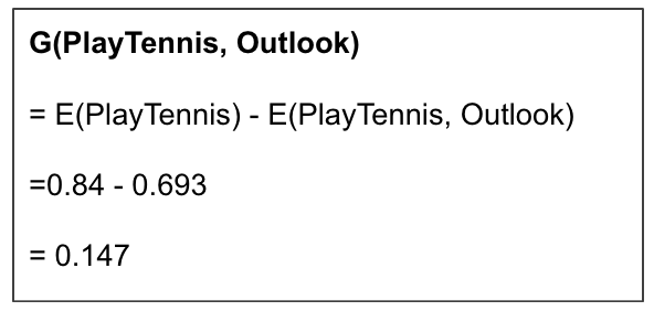
The information gain of outlook is 0.147.

sklearn.tree.DecisionTreeClassifier: “entropy” means for the information gain.

In order to visualise how to construct a decision tree using information gain, I have simply applied sklearn.tree.DecisionTreeClassifier to generate the diagram.

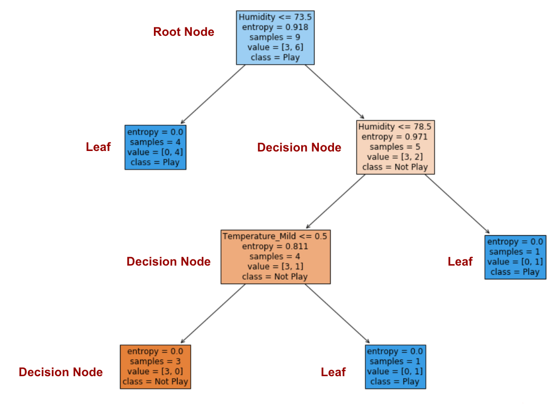
Step 3: Choose attribute with the largest Information Gain as the Root Node

The information gain of ‘Humidity’ is the highest at 0.918. Humidity is the root node.

Step 4: A branch with an entropy of 0 is a leaf node, while a branch with entropy more than 0 needs further splitting.

Step 5: Nodes are grown recursively in the ID3 algorithm until all data is classified.

You might hear of the C4.5 algorithm, an improvement of ID3 uses the Gain Ratio as an extension to information gain. The advantage of using Gain Ratio is to handle the issue of bias by normalizing the information gain using Split Info. I won’t go into details of C4.5 here. For more information, please check out here (DataCamp).

CART (Classification and Regression Tree)

Another decision tree algorithm CART uses the Gini method to create split points, including the Gini Index (Gini Impurity) and Gini Gain.

Definition of Gini Index: The probability of assigning a wrong label to a sample by picking the label randomly and is also used to measure feature importance in a tree.

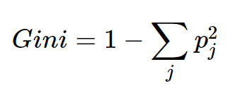
The equation of Gini Index.

Let me show you how to calculate Gini Index and Gini Gain :)

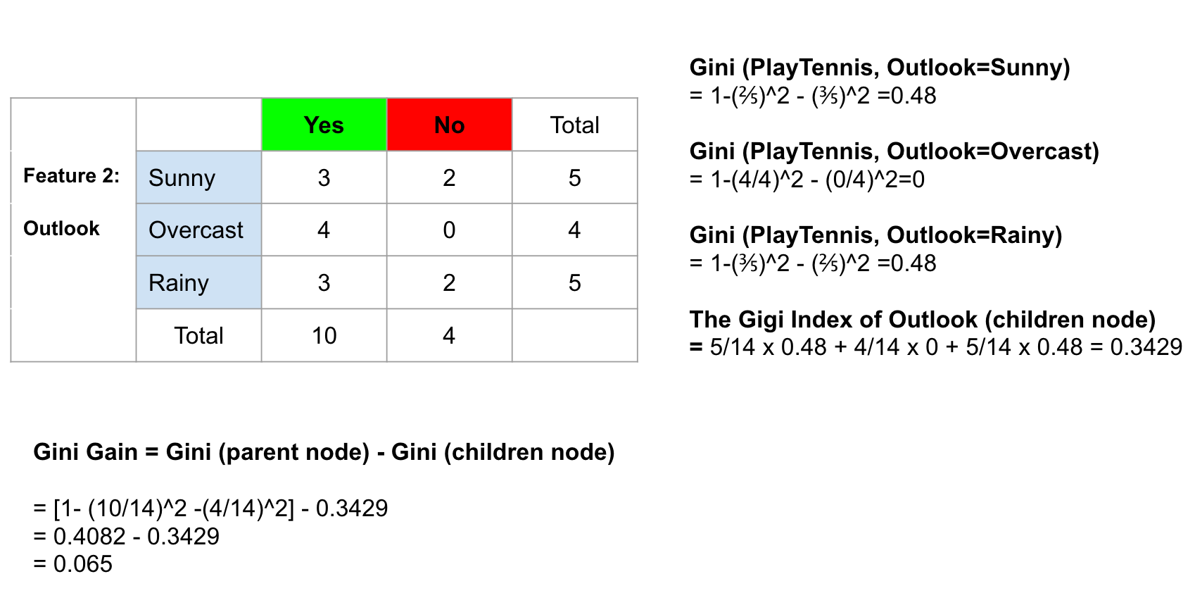
After calculating Gini Gain for every attribute, sklearn.tree.DecisionTreeClassifier will choose the attribute with the largest Gini Gain as the Root Node. A branch with Gini of 0 is a leaf node, while a branch with Gini more than 0 needs further splitting. Nodes are grown recursively until all data is classified (see the detail below).

As mentioned, CART can also handle the regression problem using a different splitting criterion: Mean Squared Error (MSE) to determine the splitting points. The output variable of a Regression Tree is numerical, and the input variables allow a mixture of continuous and categorical variables. You can check out more information about the regression trees through DataCamp.

Great! You now should understand how to calculate Entropy, Information Gain, Gini Index, and Gini Gain!

Question: so…which should I use? Gini Index or Entropy?

Answer: Generally, the result should be the same… I personally prefer Gini Index because it doesn’t involve a more computationally intensive log to calculate. But why not try both.

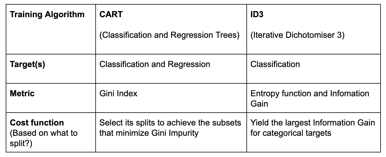
Let me summarize in a table format!

Building a Decision Tree using Scikit Learn

Scikit Learn is a free software machine learning library for the Python programming language.

Step 1: importing data

import numpy as np
import pandas as pd
df = pd.read_csv('weather.csv')

Step 2: converting categorical variables into dummies/indicator variables

df_getdummy=pd.get_dummies(data=df, columns=['Temperature', 'Outlook', 'Windy'])

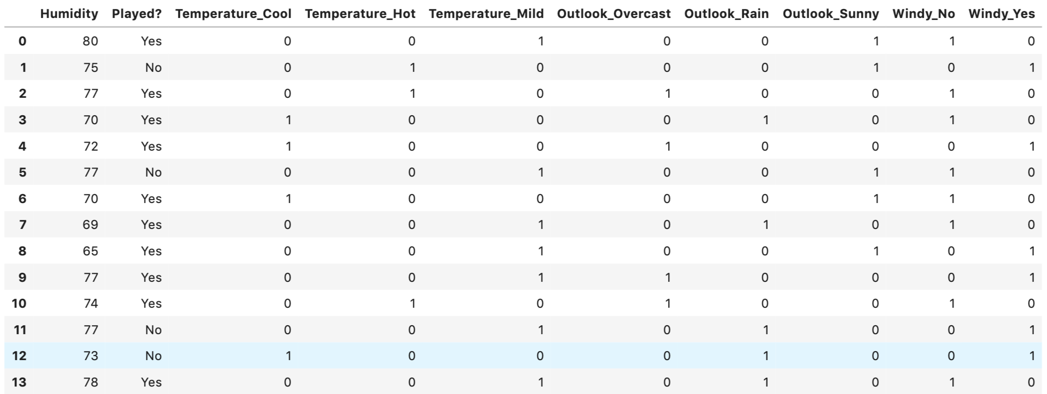
The categorical variables of ‘Temperature’, ‘Outlook’ and ‘Windy’ are all converted into dummies.

Step 3: separating the training set and test set

from sklearn.model_selection import train_test_split
X = df_getdummy.drop('Played?',axis=1)
y = df_getdummy['Played?']
X_train, X_test, y_train, y_test = train_test_split(X, y, test_size=0.30, random_state=101)

Step 4: importing Decision Tree Classifier via sklean

from sklearn.tree import DecisionTreeClassifier
dtree = DecisionTreeClassifier(max_depth=3)
dtree.fit(X_train,y_train)
predictions = dtree.predict(X_test)

Step 5: visualising the decision tree diagram

from sklearn.tree import DecisionTreeClassifier
dtree = DecisionTreeClassifier(max_depth=3)
dtree.fit(X_train,y_train)
predictions = dtree.predict(X_test)
from sklearn.tree import plot_tree
import matplotlib.pyplot as plt
fig = plt.figure(figsize=(16,12))
a = plot_tree(dtree, feature_names=df_getdummy.columns, fontsize=12, filled=True,
class_names=['Not Play', 'Play'])

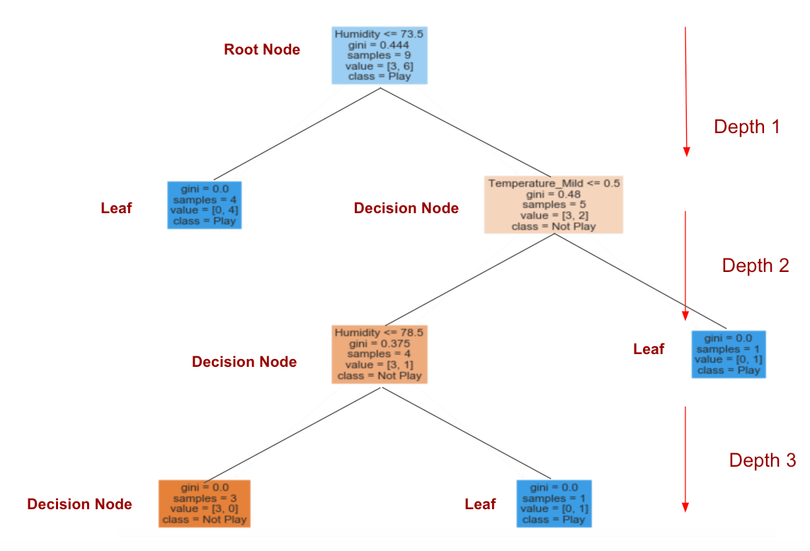
The tree depth: 3.

For the coding and dataset, please check out here.

If the condition of ‘Humidity’ is lower or equal to 73.5, it is pretty sure that Clare will play tennis!

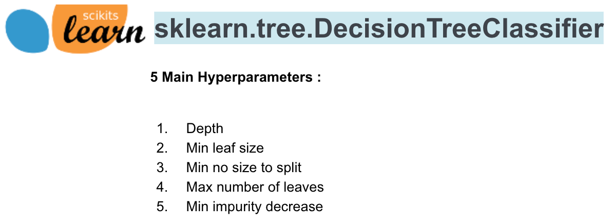
In order to improve the model performance (Hyperparameters Optimization), you should adjust the hyperparameters. For more details, please check out here.

The major disadvantage of Decision Trees is overfitting, especially when a tree is particularly deep. Fortunately, the more recent tree-based models, including random forest and XGBoost, are built on the top of the decision tree algorithm, and they generally perform better with a strong modeling technique and much more dynamic than a single decision tree. Therefore, understanding the concepts and algorithms behind Decision Trees thoroughly is super helpful in constructing a good foundation of learning data science and machine learning.

Summary: Now you should know

• How to construct a Decision Tree
• How to calculate ‘Entropy’ and ‘Information Gain’
• How to calculate the ‘Gini Index’ and ‘Gini Gain’
• What is the best split?
• How to plot a Decision Tree Diagram in Python

Original. Reposted with permission.

Related:

• Decision Tree Algorithm, Explained
• Understanding Decision Trees for Classification in Python
• Decision Trees — An Intuitive Introduction