Getting Started with Feature Selection
For machine learning, more data is always better. What about more features of data? Not necessarily. This beginners' guide with code examples for selecting the most useful features from your data will jump start you toward developing the most effective and efficient learning models.
You wouldn’t use the amount of press-ups you can do to determine the bus arrival time would you? In the same way, in predictive modelling, we prune away the non-useful features in order to reduce the complexity of the final model. Simply put, Feature selection reduces the number of input features when developing a predictive model.
In this article, I discuss the 3 main categories that feature selection falls into; filter methods, wrapper methods, and embedded methods. Additionally, I use Python examples and leverage frameworks such as scikit-learn (see the Documentation) for Machine learning, Pandas (Documentation) for data manipulation, and Plotly (Documentation) for interactive data visualization. For access to the code used in this article, visit my GitHub.

Figure 1: Clothing Rack Photo by Zui Hoang on Unsplash.
Why do Feature Selection?
The message that the first paragraph aimed to convey is that sometimes there are features that do not contribute enough useful information to predicting the final outcome, so by including it in our model, we are making our model unneededly more complex. Discarding of non-useful features results in a parsimonious model, which in turn leads to a reduced scoring time. Additionally, Feature Selection also makes interpreting models much easier, which is extremely important in most business cases.
“In most real-world cases, applying feature selection is unlikely to provide large gains in performance. However, it is still a valuable tool in the toolbox of the feature engineer.” — (Müller, (2016), Introduction to Machine Learning with Python, O’Reilley Media )
Methods
There are various methods that could be used to perform Feature Selection, of which they fall into one of 3 categories. Each method has its own advantages and disadvantages. The categories are described in Guyon & Elisseeff (2003) as follows:
- Filtering Methods- Select subsets of variables as a pre-processing step, independently of the chosen predictor.
- Wrapper Methods - Utilize the learning machine of interest as a black box to score subsets of variables according to their predictive power.
- Embedded Methods - Perform variable selection in the process of training and are usually specific to given learning machines.
Filtering Methods
Figure 2: Filtering a hot drinking Photo by Tyler Nix on Unsplash.
Filter methods use univariate statistics to evaluate whether there is a statistically significant relationship from each input feature to the target feature (target variable/dependent variable) — what we are attempting to predict. The features that provide the highest confidence are the features that we keep for our final model. Therefore, this method is independent of the choice model that we decide to use for modelling.
“Even when variable ranking is not optimal, it may be preferable to other variable subset selection methods because of its computational and statistical scalability”- Guyon and Elisseeff (2003)
An example of a filtering method is Pearson's correlation coefficient — you may have come across this in high school statistics class. This is a statistic that is used to measure the amount of linear correlation between and input X feature and the output Y feature. It ranges from +1 to -1, where 1 means there is total positive correlation, and -1 means that there is total negative correlation. Therefore, 0 is means that there is no linear correlation.
To calculate the Pearson correlation coefficient, take the covariance of the input feature X and output feature Y and divide it by the product of the two features’ standard deviation — the formula is displayed in Figure 3.
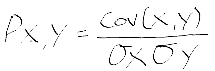
Figure 3: Formula for Pearson’s correlation coefficient where Cov is the covariance, σX is the standard deviation of X, and σY is the standard deviation of Y.
For the coding examples that follow, I use the Boston housing prices available in the Scikit-Learn framework — see Documentation — as well as Pandas for data manipulation — see Documentation.
import pandas as pd
from sklearn.datasets import load_boston

# load data
boston_bunch = load_boston()
df = pd.DataFrame(data= boston_bunch.data,
                  columns= boston_bunch.feature_names)

# adding the target variable
df["target"] = boston_bunch.target
df.head()
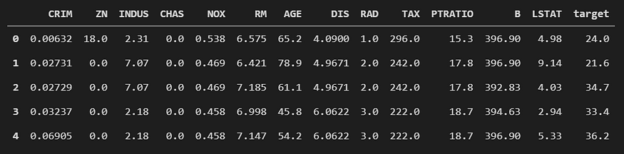
Figure 4: Output from the above code cell to display a preview of the Boston house prices dataset.
The following code is an example of the Pearson correlation coefficient for feature selection implemented in Python.
# Pearson correlation coefficient
corr = df.corr()["target"].sort_values(ascending=False)[1:]

# absolute for positive values
abs_corr = abs(corr)

# random threshold for features to keep
relevant_features = abs_corr[abs_corr>0.4]
relevant_features

>>> RM         0.695360
NOX        0.427321
TAX        0.468536
INDUS      0.483725
PTRATIO    0.507787
LSTAT      0.737663
Name: target, dtype: float64
Then, simply select the input features as follows…
new_df = df[relevant_features.index]
Advantages
- Robust against overfitting (that would introduce bias)
- Much faster than wrapper methods
Disadvantages
- Does not consider interactions between other features
- Does not consider the model being employed
Wrapper Methods
Figure 4: Wrapping a box; Photo by Kira auf der Heide on Unsplash.
Wikipedia describes Wrapper methods as using a “predictive model to score feature subsets. Each new subset is used to train a model, which is tested on a hold-out set. Counting the number of mistakes made on that hold-out set (the error rate of the model) gives the score for that subset.” — Wrapper Methods Wikipedia. The algorithms employed by wrapper methods are referred to as greedy because of the attempt to find the optimal combination of features that results in the best performing model.
“Wrapper feature selection methods create many models with various different subsets of the input features and select those features that result in the best performing model according to some performance metric.” — Jason Brownlee
One wrapper method is recursive feature elimination (RFE), and, as the name of the algorithm suggests, it works by recursively removing features, then builds a model using the remaining features and calculates the accuracy of the model.
Documentation for RFE implementation in scikit-learn.
from sklearn.feature_selection import RFE
from sklearn.linear_model import LinearRegression

# input and output features
X = df.drop("target", axis= 1)
y = df["target"]

# defining model to build
lin_reg = LinearRegression()

# create the RFE model and select 6 attributes
rfe = RFE(lin_reg, 6)
rfe.fit(X, y)

# summarize the selection of the attributes
print(f"Number of selected features: {rfe.n_features_}\n\
Mask: {rfe.support_}\n\
Selected Features:", [feature for feature, rank in zip(X.columns.values, rfe.ranking_) if rank==1],"\n\
Estimator : {rfe.estimator_}")
The print statement below returns…
Number of selected features: 6

Mask: [False False False  True  True  True False  True False False  True False   True]

Selected Features: ['CHAS', 'NOX', 'RM', 'DIS', 'PTRATIO', 'LSTAT']

Estimator : {rfe.estimator_}
Advantages
- Able to detect the interactions that take place between features
- Often results in better predictive accuracy than filter methods
- Finds the optimal feature subset
Disadvantages
- Computationally expensive
- Prone to overfitting
Embedded Methods
Figure 5: Embedded components; Photo by Chris Ried on Unsplash.
Embedded methods are similar to Wrapper methods because this method also optimizes an objective function of a predictive model, but what separates the two methods is that in embedded methods, there is an intrinsic metric used during learning to build the model. Therefore, Embedded methods require a supervised learning model, which in turn will intrinsically determine the importance of each feature for predicting the target feature.
Note: The model that is used for feature selection does not have to be the model that is used as the final model.
LASSO (Least Absolute Shrinkage and Selection Operator) is a good example of an embedded method. Wikipedia describes LASSO as “a regression analysis method that performs both variable selection and regularization in order to enhance the prediction accuracy and interpretability of the statistical model it produces.” Going into depth about how LASSO works is beyond the scope of this article, but a good article to get to grips with the algorithm can be found on the Analytics Vidhya blog by Aarshay Jain titled A Complete Tutorial on Ridge and Lasso Regression in Python.
# train model
lasso = Lasso()
lasso.fit(X, y)

# perform feature selection
kept_cols = [feature for feature, weight in zip(X.columns.values, lasso.coef_) if weight != 0]

kept_cols
This returns the columns that the Lasso regression model thought was relevant…
['CRIM', 'ZN', 'RM', 'AGE', 'DIS', 'RAD', 'TAX', 'PTRATIO', 'B', 'LSTAT']
We can also use a waterfall chart to visualize the coefficients…
figt = go.Figure(
         go.Waterfall(name= "Lasso Coefficients",
                      orientation= "h",
                      y = X.columns.values,
                      x = lasso.coef_))

fig.update_layout(title = "Coefficients of Lasso Regression Model")

fig.show()
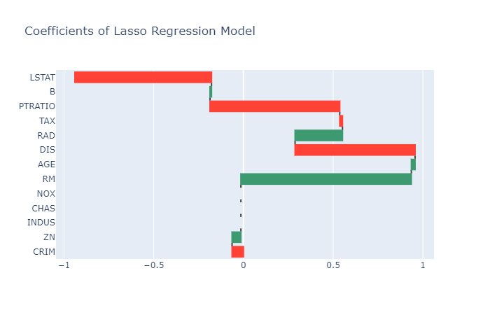
Figure 6: Output of prior code; Waterfall chart displays coefficients from feature to feature; Note that 3 features have been set to 0, meaning that they were disregarded by the model.
Advantages
- Computationally much faster than wrapper methods
- More accurate than filter methods
- Considers all the features at one time
- Not prone to overfitting
Disadvantages
- Selects features that are specific to the model
- Not as powerful as wrapper methods
Tip: There is no best feature selection method. What works well for one business use case may not work for another, so it is down to you to conduct experiments and see what works best.
Conclusion
In this article, I introduced different methods for performing feature selection. Of course, there are other ways you could do feature selection such as ANOVA, backward feature elimination, and using a decision tree. For a good article to learn more about those methods, I suggest reading Madeline McCombe’s article titled Intro to Feature Selection methods for Data Science.
Original. Reposted with permission.
Related: