 4 ways to improve your TensorFlow model – key regularization techniques you need to know
 4 ways to improve your TensorFlow model – key regularization techniques you need to know
Regularization techniques are crucial for preventing your models from overfitting and enables them perform better on your validation and test sets. This guide provides a thorough overview with code of four key approaches you can use for regularization in TensorFlow.

Photo by Jungwoo Hong on Unsplash.
Reguaralization
According to Wikipedia,
In mathematics, statistics, and computer science, particularly in machine learning and inverse problems, regularization is the process of adding information in order to solve an ill-posed problem or to prevent overfitting.
This means that we add some extra information in order to solve a problem and to prevent overfitting.
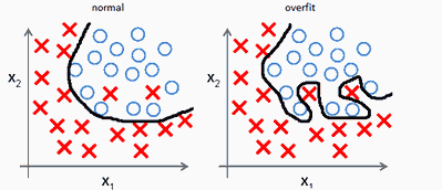
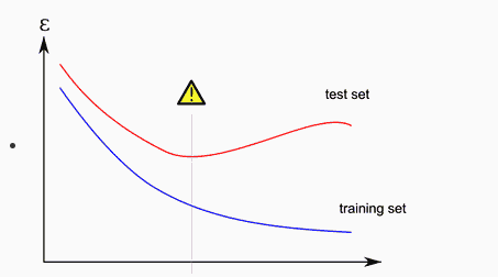
Overfitting simply means that our Machine Learning Model is trained on some data, and it will work extremely well on that data, but it will fail to generalize on new unseen examples.
We can see overfitting in this simple example
http://mlwiki.org/index.php/Overfitting
Where our data is strictly attached to our training examples. This results in poor performance on test/dev sets and good performance on the training set.
http://mlwiki.org/index.php/Overfitting
So in order to improve the performance of the model, we use different regularization techniques. There are several techniques, but we will discuss 4 main techniques.
- L1 Regularization
- L2 Regularization
- Dropout
- Batch Normalization
I will briefly explain how these techniques work and how to implement them in Tensorflow 2.
In order to get good intuition about how and why they work, I refer you to Professor Andrew NG lectures on all these topics, easily available on Youtube.
First, I will code a model without Regularization, then I will show how to improve it by adding different regularization techniques. We will use the IRIS data set to show that using regularization improves the same model a lot.
Model without Regularization
Code:
- Basic Pre-processing
- Model Building
model1.summary()
Model: "sequential"
_________________________________________________________________
Layer (type)                 Output Shape              Param #
=================================================================
dense_6 (Dense)              (None, 512)               2560
_________________________________________________________________
dense_7 (Dense)              (None, 256)               131328
_________________________________________________________________
dense_8 (Dense)              (None, 128)               32896
_________________________________________________________________
dense_9 (Dense)              (None, 64)                8256
_________________________________________________________________
dense_10 (Dense)             (None, 32)                2080
_________________________________________________________________
dense_11 (Dense)             (None, 3)                 99
=================================================================
Total params: 177,219
Trainable params: 177,219
Non-trainable params: 0
_________________________________________________________________
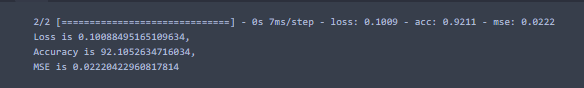
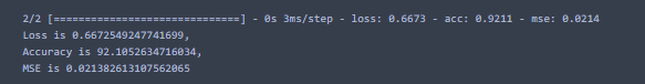
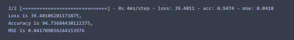
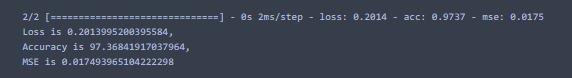
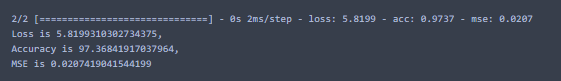
After training the model, if we evaluate the model using the following code in Tensorflow, we can find our accuracy, loss, and mse at the test set.
loss1, acc1, mse1 = model1.evaluate(X_test, y_test)
print(f"Loss is {loss1},\nAccuracy is {acc1*100},\nMSE is {mse1}")
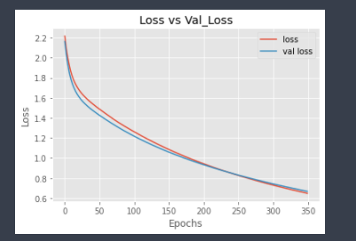
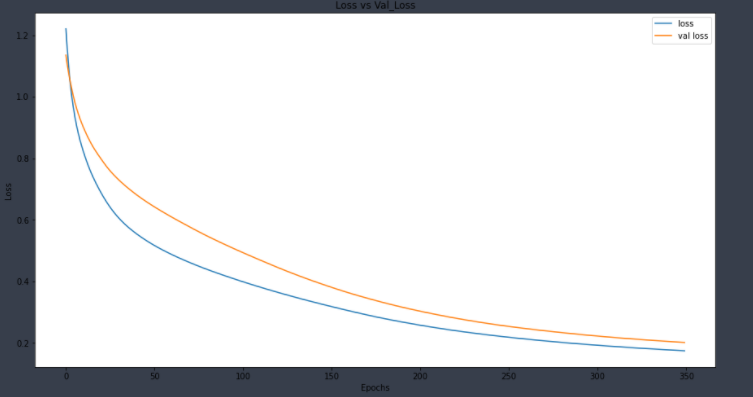
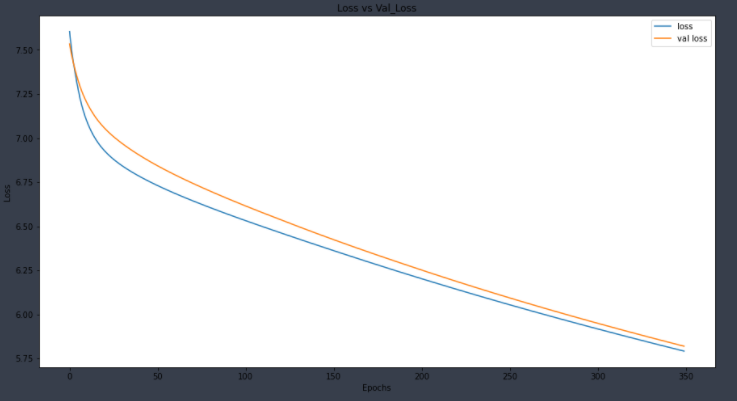
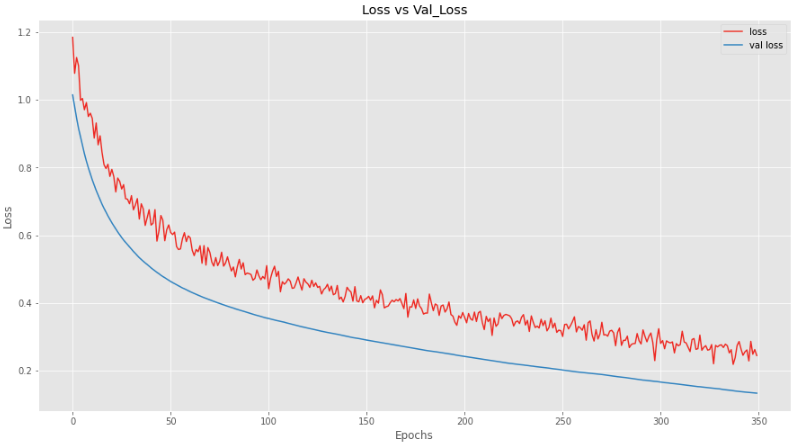
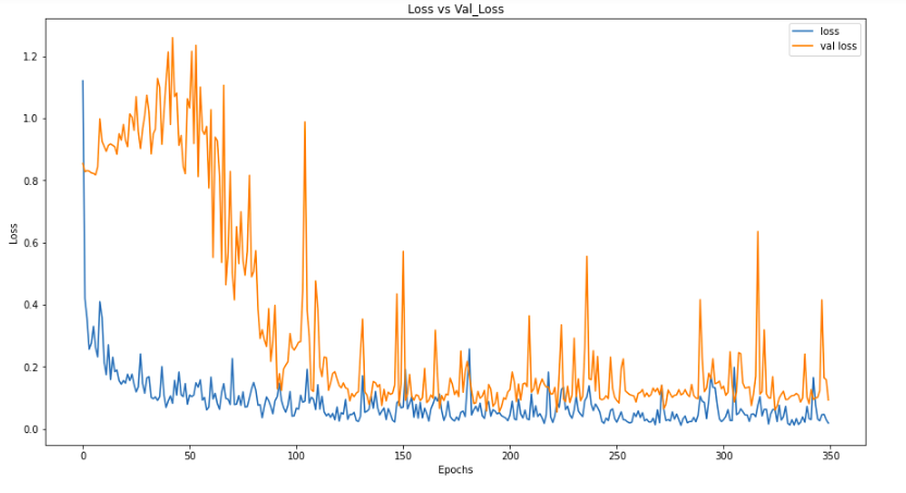
Let’s check the plots for Validation Loss and Training Loss.
import matplotlib.pyplot as plt
plt.style.use('ggplot')
plt.plot(hist.history['loss'], label = 'loss')
plt.plot(hist.history['val_loss'], label='val loss')
plt.title("Loss vs Val_Loss")
plt.xlabel("Epochs")
plt.ylabel("Loss")
plt.legend()
plt.show()
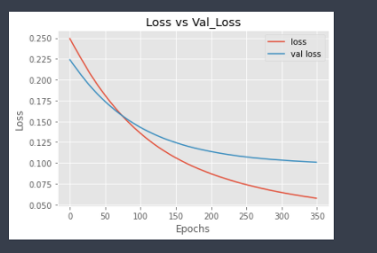
Here, we can see that validation loss is gradually increasing after ≈ 60 epochs as compared to training loss. This shows that our model is overfitted.
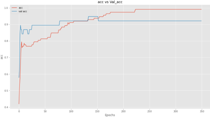
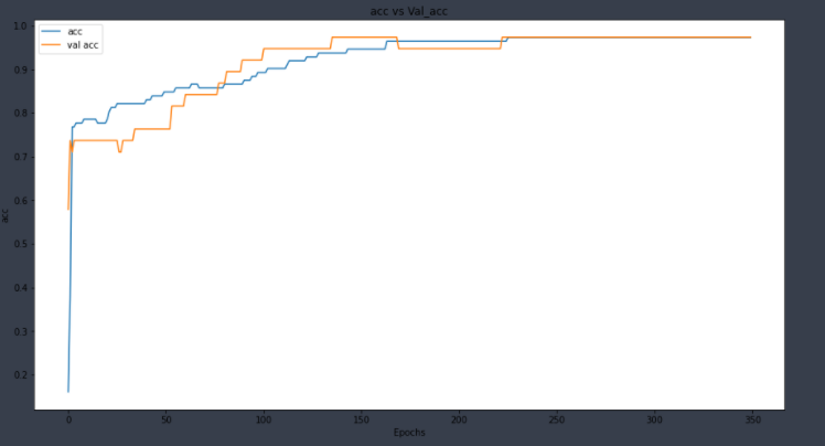
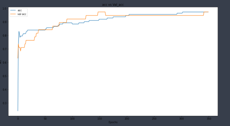
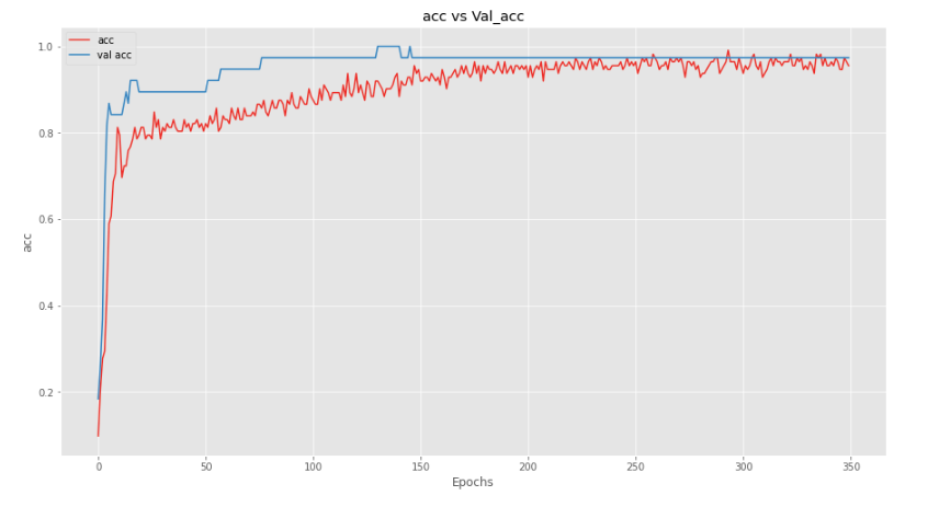
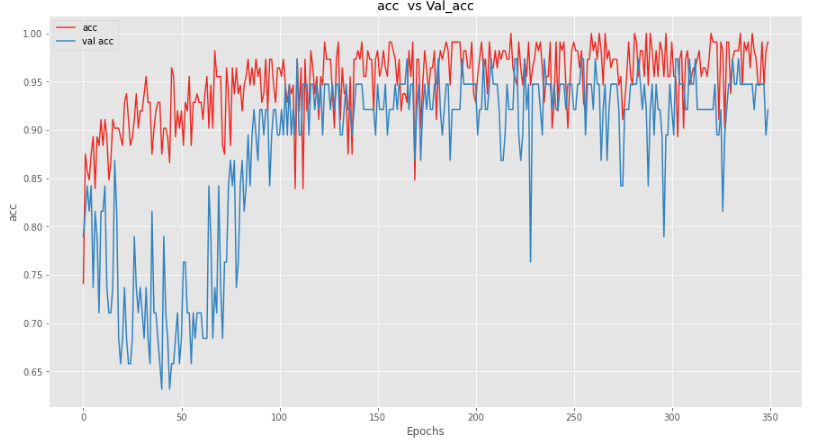
And similarly, for model accuracy plot,
plt.plot(hist.history['acc'], label = 'acc')
plt.plot(hist.history['val_acc'], label='val acc')
plt.title("acc vs Val_acc")
plt.xlabel("Epochs")
plt.ylabel("acc")
plt.legend()
plt.show()
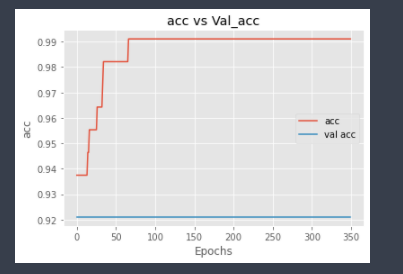
This again shows that validation accuracy is low as compared to training accuracy, which again shows signs of overfitting.
L1 Regularization:
A commonly used Regularization technique is L1 regularization, also known as Lasso Regularization.
The main concept of L1 Regularization is that we have to penalize our weights by adding absolute values of weight in our loss function, multiplied by a regularization parameter lambda λ, where λ is manually tuned to be greater than 0.
The equation for L1 is
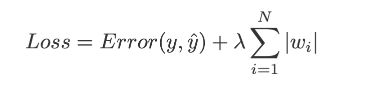
Image Credit: Towards Data Science.
Tensorflow Code:
Here, we added an extra parameter kernel_regularizer, which we set it to ‘l1’ for L1 Regularization.
Let’s Evaluate and plot the model now.
loss2, acc2, mse2 = model2.evaluate(X_test, y_test)
print(f"Loss is {loss2},\nAccuracy is {acc2 * 100},\nMSE is {mse2}")
Hmmm, Accuracy is pretty much the same, let’s check the plots to get better intuition.
plt.plot(hist2.history[‘loss’], label = ‘loss’)
plt.plot(hist2.history[‘val_loss’], label=’val loss’)
plt.title(“Loss vs Val_Loss”)
plt.xlabel(“Epochs”)
plt.ylabel(“Loss”)
plt.legend()
plt.show()
And for Accuracy,
plt.figure(figsize=(15,8))
plt.plot(hist2.history['acc'], label = 'acc')
plt.plot(hist2.history['val_acc'], label='val acc')
plt.title("acc vs Val_acc")
plt.xlabel("Epochs")
plt.ylabel("acc")
plt.legend()
plt.show()
Well, quite an improvement, I guess, because over validation loss is not increasing that much as it was previously, but validation accuracy is not increasing much. Let’s add l1 in more layers to check if it improves the model or not.
model3 = Sequential([
    Dense(512, activation='tanh', input_shape = X_train[0].shape, kernel_regularizer='l1'),
    Dense(512//2, activation='tanh', kernel_regularizer='l1'),
    Dense(512//4, activation='tanh', kernel_regularizer='l1'),
    Dense(512//8, activation='tanh', kernel_regularizer='l1'),
    Dense(32, activation='relu', kernel_regularizer='l1'),
    Dense(3, activation='softmax')
])
model3.compile(optimizer='sgd',loss='categorical_crossentropy', metrics=['acc', 'mse'])
hist3 = model3.fit(X_train, y_train, epochs=350, batch_size=128, validation_data=(X_test,y_test), verbose=2)
After training, let’s evaluate the model.
loss3, acc3, mse3 = model3.evaluate(X_test, y_test)
print(f"Loss is {loss3},\nAccuracy is {acc3 * 100},\nMSE is {mse3}")
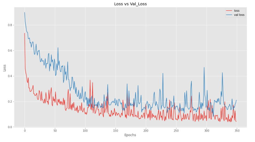
Well, the accuracy is quite improved now, it jumped from 92 to 94. Let’s check the plots.
Loss
plt.figure(figsize=(15,8))
plt.plot(hist3.history['loss'], label = 'loss')
plt.plot(hist3.history['val_loss'], label='val loss')
plt.title("Loss vs Val_Loss")
plt.xlabel("Epochs")
plt.ylabel("Loss")
plt.legend()
plt.show()
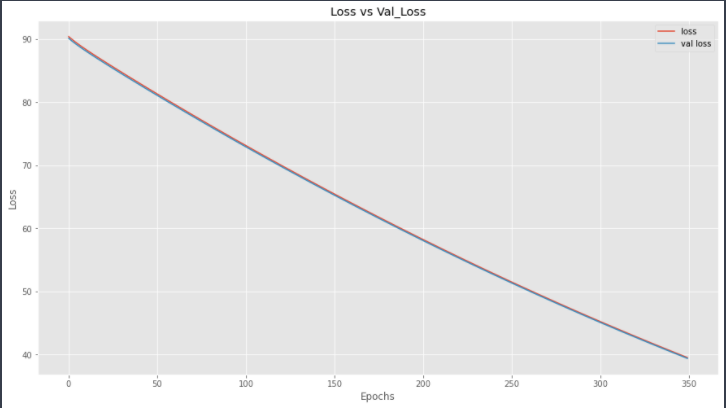
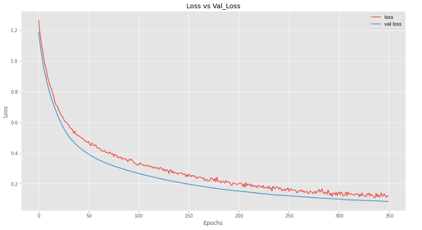
Now, both lines are approximately overlapping, which means that our model is performing just as same on the test set as it was performing on the training set.
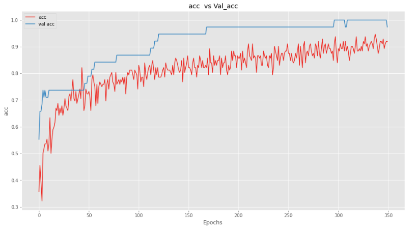
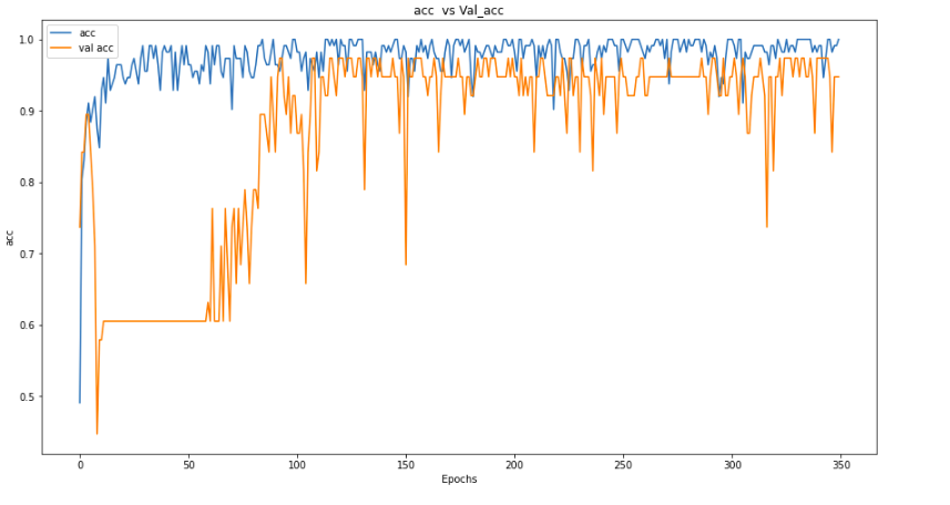
Accuracy
plt.figure(figsize=(15,8))
plt.plot(hist3.history['acc'], label = 'ACC')
plt.plot(hist3.history['val_acc'], label='val acc')
plt.title("acc vs Val_acc")
plt.xlabel("Epochs")
plt.ylabel("acc")
plt.legend()
plt.show()
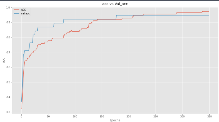
And we can see that the validation loss of the model is not increasing as compared to training loss, and validation accuracy is also increasing.
L2 Regularization
L2 Regularization is another regularization technique which is also known as Ridge regularization. In L2 regularization we add the squared magnitude of weights to penalize our lost function.
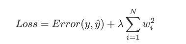
Image Credit: Towards Data Science.
Tensorflow Code:
model5 = Sequential([
    Dense(512, activation='tanh', input_shape = X_train[0].shape, kernel_regularizer='l2'),
    Dense(512//2, activation='tanh'),
    Dense(512//4, activation='tanh'),
    Dense(512//8, activation='tanh'),
    Dense(32, activation='relu'),
    Dense(3, activation='softmax')
])
model5.compile(optimizer='sgd',loss='categorical_crossentropy', metrics=['acc', 'mse'])
hist5 = model5.fit(X_train, y_train, epochs=350, batch_size=128, validation_data=(X_test,y_test), verbose=2)
After training, let’s evaluate the model.
loss5, acc5, mse5 = model5.evaluate(X_test, y_test)
print(f"Loss is {loss5},\nAccuracy is {acc5 * 100},\nMSE is {mse5}")
And the output is
Here we can see that validation accuracy is 97%, which is quite good. Let’s plot for more intuition.
Here we can see that we are not overfitting our data. Let’s plot accuracy.
Adding “L2” Regularization in just 1 layer has improved our model a lot.
Let’s Now add L2 in all other layers.
model6 = Sequential([
    Dense(512, activation='tanh', input_shape = X_train[0].shape, kernel_regularizer='l2'),
    Dense(512//2, activation='tanh', kernel_regularizer='l2'),
    Dense(512//4, activation='tanh', kernel_regularizer='l2'),
    Dense(512//8, activation='tanh', kernel_regularizer='l2'),
    Dense(32, activation='relu', kernel_regularizer='l2'),
    Dense(3, activation='softmax')
])
model6.compile(optimizer='sgd',loss='categorical_crossentropy', metrics=['acc', 'mse'])
hist6 = model6.fit(X_train, y_train, epochs=350, batch_size=128, validation_data=(X_test,y_test), verbose=2)
Here we have L2 in all layers. After training, let’s evaluate it.
loss6, acc6, mse6 = model6.evaluate(X_test, y_test)
print(f"Loss is {loss6},\nAccuracy is {acc6 * 100},\nMSE is {mse6}")
Let’s plot to get more intuitions.
plt.figure(figsize=(15,8))
plt.plot(hist6.history['loss'], label = 'loss')
plt.plot(hist6.history['val_loss'], label='val loss')
plt.title("Loss vs Val_Loss")
plt.xlabel("Epochs")
plt.ylabel("Loss")
plt.legend()
plt.show()
And for accuracy
We can see that this model is also good and not overfitting to the dataset.
Dropout
Another common way to avoid regularization is by using the Dropout technique. The main idea behind using dropout is that we randomly turn off some neurons in our layer based on some probability. You can learn more about it’s working by Professor NG’s video here.
Let’s code it in Tensorflow.
All previous imports are the same, and we are just adding an extra import here.
In order to implement DropOut, all we have to do is to add a Dropout layer from tf.keras.layers and set a dropout rate in it.
import tensorflow as tf
model7 = Sequential([
    Dense(512, activation='tanh', input_shape = X_train[0].shape),
    tf.keras.layers.Dropout(0.5), #dropout with 50% rate
    Dense(512//2, activation='tanh'),

    Dense(512//4, activation='tanh'),
    Dense(512//8, activation='tanh'),
    Dense(32, activation='relu'),
    Dense(3, activation='softmax')
])
model7.compile(optimizer='sgd',loss='categorical_crossentropy', metrics=['acc', 'mse'])
hist7 = model7.fit(X_train, y_train, epochs=350, batch_size=128, validation_data=(X_test,y_test), verbose=2)
After training, let’s evaluate it on the test set.
loss7, acc7, mse7 = model7.evaluate(X_test, y_test)
print(f"Loss is {loss7},\nAccuracy is {acc7 * 100},\nMSE is {mse7}")

And wow, our results are very promising, we performed 97% on our test set. Let’s plot the loss and accuracy for better intuition.
plt.figure(figsize=(15,8))
plt.plot(hist7.history['loss'], label = 'loss')
plt.plot(hist7.history['val_loss'], label='val loss')
plt.title("Loss vs Val_Loss")
plt.xlabel("Epochs")
plt.ylabel("Loss")
plt.legend()
plt.show()
Here, we can see that our model is performing better on validation data as compared to training data, which is good news.
Let’s plot accuracy now.
And we can see that our model is performing better on the validation dataset as compared to the training set.
Let’s add more dropout layers to see how our model performs.
model8 = Sequential([
    Dense(512, activation='tanh', input_shape = X_train[0].shape),
    tf.keras.layers.Dropout(0.5),
    Dense(512//2, activation='tanh'),
    tf.keras.layers.Dropout(0.5),
    Dense(512//4, activation='tanh'),
    tf.keras.layers.Dropout(0.5),
    Dense(512//8, activation='tanh'),
    tf.keras.layers.Dropout(0.3),
    Dense(32, activation='relu'),
    Dense(3, activation='softmax')
])
model8.compile(optimizer='sgd',loss='categorical_crossentropy', metrics=['acc', 'mse'])
hist8 = model8.fit(X_train, y_train, epochs=350, batch_size=128, validation_data=(X_test,y_test), verbose=2)
Let’s Evaluate it.
loss8, acc8, mse8 = model8.evaluate(X_test, y_test)
print(f"Loss is {loss8},\nAccuracy is {acc8 * 100},\nMSE is {mse8}")

This model is also very good, as it is performing 98% on the test set. Let’s plot to get better intuitions.
plt.figure(figsize=(15,8))
plt.plot(hist8.history['loss'], label = 'loss')
plt.plot(hist8.history['val_loss'], label='val loss')
plt.title("Loss vs Val_Loss")
plt.xlabel("Epochs")
plt.ylabel("Loss")
plt.legend()
plt.show()
And we can see that adding more dropout layers makes the model perform slightly less good while training, but on the validation set, it is performing really well.
Let’s plot the accuracy now.
And we can see the same pattern here, that our model is not performing as good while training, but when we are evaluating it, it is performing really good.
Batch Normalization
The main idea behind batch normalization is that we normalize the input layer by using several techniques (sklearn.preprocessing.StandardScaler) in our case, which improves the model performance, so if the input layer is benefitted by normalization, why not normalize the hidden layers, which will improve and fasten learning even further.
To learn maths and get more intuition about it, I will redirect you again to Professor NG’s lecture here and here.
To add it in your TensorFlow model, just add tf.keras.layers.BatchNormalization() after your layers.
Let’s see the code.
model9 = Sequential([
    Dense(512, activation='tanh', input_shape = X_train[0].shape),
    Dense(512//2, activation='tanh'),
    tf.keras.layers.BatchNormalization(),
    Dense(512//4, activation='tanh'),
    Dense(512//8, activation='tanh'),
    Dense(32, activation='relu'),
    Dense(3, activation='softmax')
])
model9.compile(optimizer='sgd',loss='categorical_crossentropy', metrics=['acc', 'mse'])
hist9 = model9.fit(X_train, y_train, epochs=350,  validation_data=(X_test,y_test), verbose=2)
Here, if you noticed that I have removed the option for batch_size. This is because adding batch_size argument while only using tf.keras.BatchNormalization() as regularization, this results in a really poor performance of the model. I have tried to find the reason for this on the internet, but I could not find it. You can also change the optimizer from sgd to rmsprop or adam if you really want to use batch_size while training.
After training, let’s evaluate the model.
loss9, acc9, mse9 = model9.evaluate(X_test, y_test)
print(f"Loss is {loss9},\nAccuracy is {acc9 * 100},\nMSE is {mse9}")

Validation accuracy for 1 Batch Normalization accuracy is not as good as compared to other techniques. Let’s plot the loss and acc for better intuition.
Here we can see that our model is not performing as well on validation set as on test set. Let’s add normalization to all the layers to see the results.
model11 = Sequential([
    Dense(512, activation='tanh', input_shape = X_train[0].shape),
    tf.keras.layers.BatchNormalization(),
    Dense(512//2, activation='tanh'),
    tf.keras.layers.BatchNormalization(),
    Dense(512//4, activation='tanh'),
    tf.keras.layers.BatchNormalization(),
    Dense(512//8, activation='tanh'),
    tf.keras.layers.BatchNormalization(),
    Dense(32, activation='relu'),
    tf.keras.layers.BatchNormalization(),
    Dense(3, activation='softmax')
])
model11.compile(optimizer='sgd',loss='categorical_crossentropy', metrics=['acc', 'mse'])
hist11 = model11.fit(X_train, y_train, epochs=350,  validation_data=(X_test,y_test), verbose=2)
Let’s Evaluate it.
loss11, acc11, mse11 = model11.evaluate(X_test, y_test)
print(f"Loss is {loss11},\nAccuracy is {acc11 * 100},\nMSEis {mse11}")

By adding Batch normalization in every layer, we achieved good accuracy. Let’s plot the loss and accuracy.
By plotting accuracy and loss, we can see that our model is still performing better on the Training set as compared to the validation set, but still, it is improving in performance.
Outcome:
This article was a brief introduction on how to use different techniques in Tensorflow. If you lack the theory, I would suggest Course 2 and 3 of Deep Learning Specialization at Coursera to learn more about Regularization.
You also have to learn when to use which technique, and when and how to combine different techniques in order to produce really fruitful results.
Hopefully, now you have an idea of how to implement different regularization techniques in Tensorflow 2.
Related: