 Implementing a Deep Learning Library from Scratch in Python
 Implementing a Deep Learning Library from Scratch in Python
A beginner’s guide to understanding the fundamental building blocks of deep learning platforms.
By Parmeet Bhatia, Machine Learning Practitioner and Deep Learning Enthusiast
Deep Learning has evolved from simple neural networks to quite complex architectures in a short span of time. To support this rapid expansion, many different deep learning platforms and libraries are developed along the way. One of the primary goals for these libraries is to provide easy to use interfaces for building and training deep learning models, that would allow users to focus more on the tasks at hand. To achieve this, it may require to hide core implementation units behind several abstraction layers that make it difficult to understand basic underlying principles on which deep learning libraries are based. Hence the goal of this article is to provide insights on building blocks of deep learning library. We first go through some background on Deep Learning to understand functional requirements and then walk through a simple yet complete library in python using NumPy that is capable of end-to-end training of neural network models (of very simple types). Along the way, we will learn various components of a deep learning framework. The library is just under 100 lines of code and hence should be fairly easy to follow. The complete source code can be found at https://github.com/parmeet/dll_numpy
Background
Typically a deep learning computation library (like TensorFlow and PyTorch) consists of components shown in the figure below.
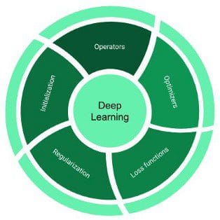
Operators
Also used interchangeably with layers, they are the basic building blocks of any neural network. Operators are vector-valued functions that transform the data. Some commonly used operators are layers like linear, convolution, and pooling, and activation functions like ReLU and Sigmoid.
Optimizers
They are the backbones of any deep learning library. They provide the necessary recipe to update model parameters using their gradients with respect to the optimization objective. Some well-known optimizers are SGD, RMSProp, and Adam.
Loss Functions
They are closed-form and differentiable mathematical expressions that are used as surrogates for the optimization objective of the problem at hand. For example, cross-entropy loss and Hinge loss are commonly used loss functions for the classification tasks.
Initializers
They provide the initial values for the model parameters at the start of training. Initialization plays an important role in training deep neural networks, as bad parameter initialization can lead to slow or no convergence. There are many ways one can initialize the network weights like small random weights drawn from the normal distribution. You may have a look at https://keras.io/initializers/ for a comprehensive list.
Regularizers
They provide the necessary control mechanism to avoid overfitting and promote generalization. One can regulate overfitting either through explicit or implicit measures. Explicit methods impose structural constraints on the weights, for example, minimization of their L1-Norm and L2-Norm that make the weights sparser and uniform respectively. Implicit measures are specialized operators that do the transformation of intermediate representations, either through explicit normalization, for example, BatchNorm, or by changing the network connectivity, for example, DropOut and DropConnect.
The above-mentioned components basically belong to the front-end part of the library. By front-end, I mean the components that are exposed to the user for them to efficiently design neural network architectures. On the back-end side, these libraries provide support for automatically calculating gradients of the loss function with respect to various parameters in the model. This technique is commonly referred to as Automatic Differentiation (AD).
Automatic Differentiation (AD)
Every deep learning library provides a flavor of AD so that a user can focus on defining the model structure (computation graph)and delegate the task of gradients computation to the AD module. Let us go through an example to see how it works. Say we want to calculate partial derivatives of the following function with respect to its input variables X₁ and X₂:
Y = sin(x₁)+X₁*X₂The following figure, which I have borrowed from https://en.wikipedia.org/wiki/Automatic_differentiation, shows it’s computation graph and calculation of derivatives via chain-rule.
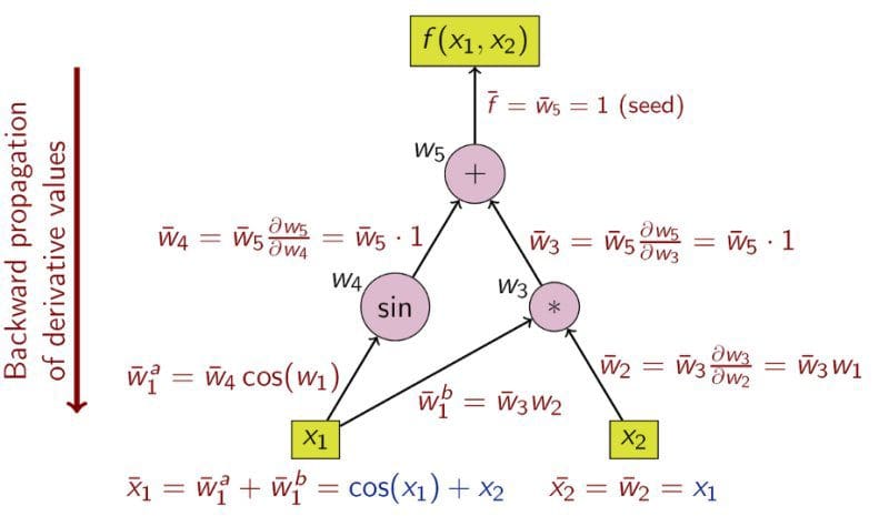
What you see in the above figure is a flavor of reverse-mode automatic differentiation (AD). The well known Back-propagation algorithm is a special case of the above algorithm where the function at the top is loss function. AD exploits the fact that every composite function consists of elementary arithmetic operations and elementary functions, and hence the derivatives can be computed by recursively applying the chain-rule to these operations.
Implementation
In the previous section, we have gone through all the necessary components to come up with our first deep learning library that can do end-to-end training. To keep things simple, I will mimic the design pattern of the Caffe Library. Here we define two abstract classes: A “Function” class and an “Optimizer” class. In addition, there is a “Tensor” class which is a simple structure containing two NumPy multi-dimensional arrays, one for holding the value of parameters and another for holding their gradients. All the parameters in various layers/operators will be of type “Tensor”. Before we dig deeper, the following figure provides a high-level overview of the library.
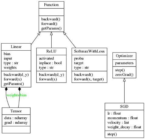
At the time of this writing, the library comes with the implementation of the linear layer, ReLU activation, and SoftMaxLoss Layer along with the SGD optimizer. Hence the library can be used to train a classification model comprising of fully connected layers and ReLU non-linearity. Lets now go through some details of the two abstract classes we have.
The “Function” abstract class provides an interface for operators and is defined as follows:
All the operators are implemented by inheriting the “Function” abstract class. Each operator must provide an implementation of forward(…) and backward(…) methods and optionally implement getParams function to provide access to its parameters (if any). The forward(…) method receives the input and returns its transformation by the operator. It will also do any house-keeping necessary to compute the gradients. The backward(…) method receives partial derivatives of the loss function with respect to the operator’s output and implements the partial derivatives of loss with respect to the operator’s input and parameters (if there are any). Note that backward(…) function essentially provides the capability for our library to perform automatic differentiation.
To make things concrete let’s look at the implementation of the Linear function as shown in the following code snippet:
The forward(…) function implements the transformation of the form Y = X*W+b and returns it. It also stores the input X as this is needed to compute the gradients of W in the backward function. The backward(…) function receives partial derivatives dY of loss with respect to the output Y and implements the partial derivatives with respect to input X and parameters W and b. Furthermore, it returns the partial derivatives with respect to the input X, that will be passed on to the previous layer.
The abstract “Optimizer” class provides an interface for optimizers and is defined as follows:
All the optimizers are implemented by inheriting the “Optimizer” base class. The concrete optimization class must provide the implementation for the step() function. This method updates the model parameters using their partial derivatives with respect to the loss we are optimizing. The reference to various model parameters is provided in the __init__(…) function. Note that the common functionality of resetting gradients is implemented in the base class itself.
To make things concrete, let’s look at the implementation of stochastic gradient descent (SGD) with momentum and weight decay.
Getting to the real stuff
To this end, we have all the ingredients to train a (deep) neural network model using our library. To do so, we would need the following:
- Model: This is our computation graph
- Data and Target: This is our training data
- Loss Function: Surrogate for our optimization objective
- Optimizer: To update model parameters
The following pseudo-code depicts a typical training cycle:
model #computation graph
data,target #training data
loss_fn #optimization objective
optim #optimizer to update model parameters to minimize lossRepeat:#until convergence or for predefined number of epochs
   optim.zeroGrad() #set all gradients  to zero
   output = model.forward(data) #get output from  model
   loss   = loss_fn(output,target) #calculate loss
   grad   = loss.backward() #calculate gradient of loss w.r.t output
   model.backward(grad) #calculate gradients for all the parameters
   optim.step() #update model parameters
Though not a necessary ingredient for a deep learning library, it may be a good idea to encapsulate the above functionality in a class so that we don’t have to repeat ourselves every time we need to train a new model (this is in line with the philosophy of higher-level abstraction frameworks like Keras). To achieve this, let’s define a class “Model” as shown in the following code snippet:
This class serves the following functionalities:
- Computation Graph: Through add(…) function, one can define a sequential model. Internally, the class will simply store all the operators in a list named computation_graph.
- Parameter Initialization: The class will automatically initialize model parameters with small random values drawn from uniform distribution at the start of training.
- Model Training: Through fit(…) function, the class provides a common interface to train the models. This function requires the training data, optimizer, and the loss function.
- Model Inference: Through predict(…) function, the class provides a common interface for making predictions using the trained model.
Since this class does not serve as a fundamental building block for deep learning, I implemented it in a separate module called utilities.py. Note that the fit(…) function makes use of DataGenerator Class whose implementation is also provided in the utilities.py module. This class is just a wrapper around our training data and generate mini-batches for each training iteration.
Training our first model
Let’s now go through the final piece of code that trains a neural network model using the proposed library. Inspired by the blog-post of Andrej Karapathy, I am going to train a hidden layer neural network model on spiral data. The code for generating the data and it’s visualization is available in the utilities.py file.
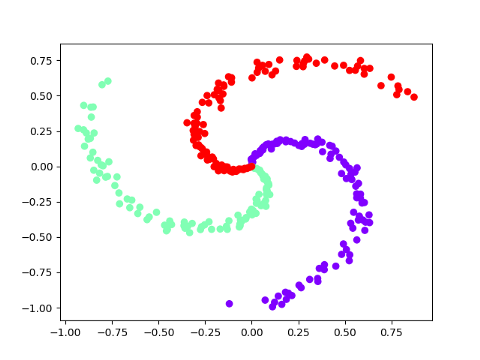
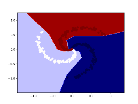
A three-class spiral data is shown in the above figure. The data is non-linearly separable. So we hope that our one hidden layer neural network can learn the non-linear decision boundary. Bringing it all together, the following code snippet will train our model.
The following figure shows the same spiral data together with the decision boundaries of the trained model.
Concluding remarks
With the ever-increasing complexity of deep learning models, the libraries tend to grow at exponential rates both in terms of functionalities and their underlying implementation. That said, the very core functionalities can still be implemented in a relatively small number of lines of code. Although the library can be used to train end-to-end neural network models (of very simple types), it is still restricted in many ways that make deep learning frameworks usable in various domains including (but not limited to) vision, speech, and text. With that said, I think this is also an opportunity to fork the base implementation and add missing functionalities to get your hands-on experience. Some of the things you can try to implement are:
- Operators: Convolution Pooling etc.
- Optimizers: Adam RMSProp etc.
- Regularizers: BatchNorm DropOut etc.
I hope this article gives you a glimpse of what happens under the hood when you use any deep learning library to train your models. Thank you for your attention and I look forward to your comments or any questions in the comment section.
Bio: Parmeet Bhatia is a Machine learning practitioner and deep learning enthusiast. He is an experienced Machine Learning Engineer and R&D professional with a demonstrated history of developing and productization of ML and data-driven products. He is highly passionate about building end-to-end intelligent systems at scale.
Original. Reposted with permission.
Related:
- Autograd: The Best Machine Learning Library You’re Not Using?
- 10 Things You Didn’t Know About Scikit-Learn
- Deep Learning for Signal Processing: What You Need to Know