Looking Inside The Blackbox: How To Trick A Neural Network

In this tutorial, I’ll show you how to use gradient ascent to figure out how to misclassify an input.

By William Falcon, Founder PyTorch Lightning

Neural networks get a bad reputation for being black boxes. And while it certainly takes creativity to understand their decision making, they are really not as opaque as people would have you believe.

In this tutorial, I’ll show you how to use backpropagation to change the input as to classify it as whatever you would like.

Follow along using this colab.

(This work was co-written with Alfredo Canziani ahead of an upcoming video)

Humans as black boxes

Let’s consider the case of humans. If I show you the following input:

there’s a good chance you have no idea whether this is a 5 or a 6. In fact, I believe that I could even make a case for convincing you that this might also be an 8.

Now, if you asked a human what they would have to do to make something more into a 5 you might visually do something like this:

And if I wanted you to make this more into an 8, you might do something like this:

Now, the answer to this question is not easy to explain in a few if statements or by looking at a few coefficients (yes, I’m looking at you regression). Unfortunately, with certain types of inputs (images, sound, video, etc…) explainability certainly becomes much harder but not impossible.

Asking the neural network

How would a neural network answer the same questions I posed above? Well, to answer that, we can use gradient ascent to do exactly that.

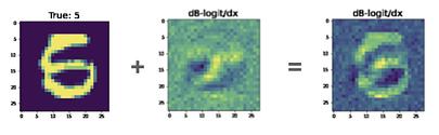
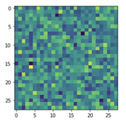
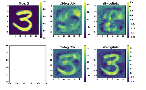
Here’s how the neural network thinks we would need to modify the input to make it more into a 5.

There are two interesting results from this. First, the black areas are where the network things we need to remove pixel density from. Second, the yellow areas are where it thinks we need to add more pixel density.

We can take a step in that gradient direction by adding the gradients to the original image. We could of course repeat this procedure over and over again to eventually morph the input into the prediction we are hoping for.

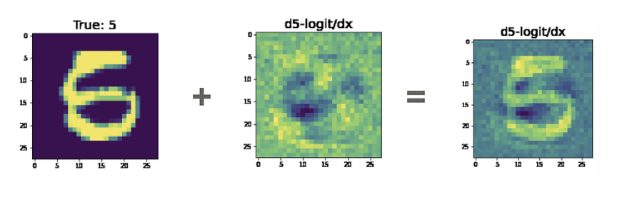
You can see that the black patch at the bottom left of the image is very similar to what a human might think to do as well.

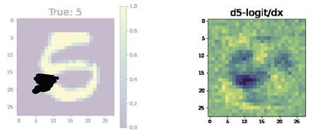
Human adds black on the left corner. Network suggests the same

What about making the input look more like an 8? Here’s how the network thinks you would have to change the input.

The notable things, here again, are that there is a black mass at the bottom left and a bright mass around the middle. If we add this with the input we get the following result:

In this case, I’m not particularly convinced that we’ve turned this 5 into an 8. However, we’ve made less of a 5, and the argument to convince you this is an 8 would certainly be easier to win using the image on the right instead of the image on the left.

Gradients are your guides

In regression analysis, we look at coefficients to tell us about what we’ve learned. In a random forest, we can look at decision nodes.

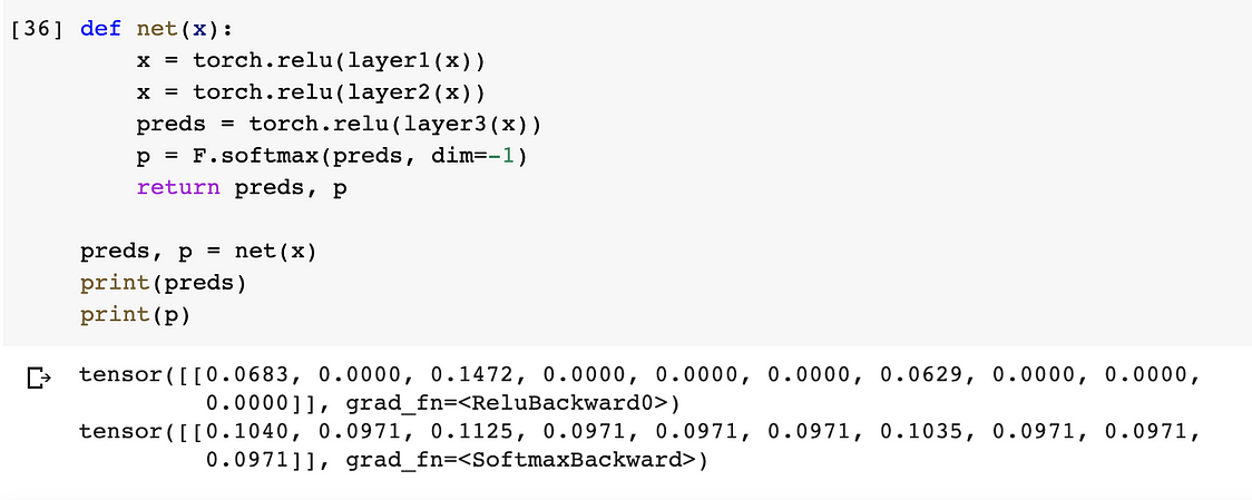
In neural networks, it comes down to how creative we are at using gradients. To classify this digit, we generated a distribution over possible predictions.

This is what we call the forward pass.

During the forward pass we calculate a probability distribution over outputs

In code it looks like this (follow along using this colab):

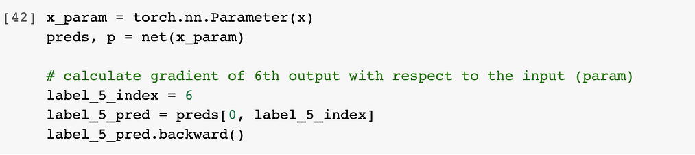
Now imagine that we wanted to trick the network into predicting “5” for the input x. Then the way to do this is to give it an image (x), calculate the predictions for the image and then maximize the probablitity of predicting the label “5”.

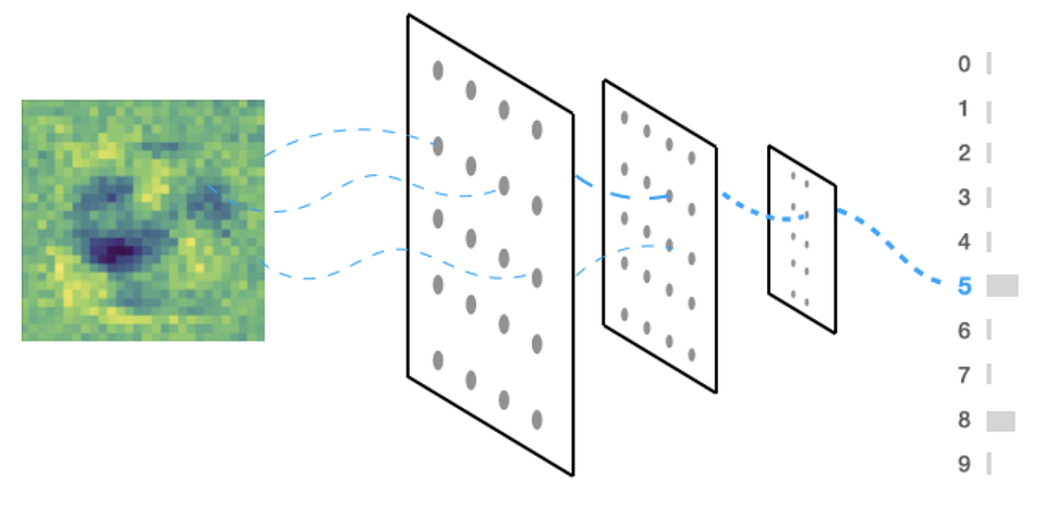
To do this we can use gradient ascent to calculate the gradients of a prediction at the 6th index (ie: label = 5) (p) with respect to the input x.

To do this in code we feed the input x as a parameter to the neural network, pick the 6th prediction (because we have labels: 0, 1, 2, 3, 4 , 5, …) and the 6th index means label “5”.

Visually this looks like:

Gradient of the prediction of a “5” with respect to the input.

And in code:

When we call .backward() the process that happens can be visualized by the previous animation.

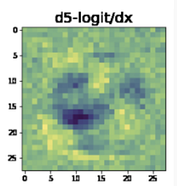
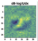
Now that we calculated the gradients, we can visualize and plot them:

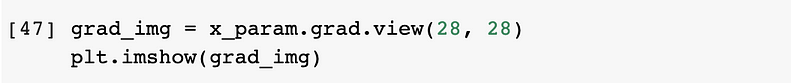
The above gradient looks like random noise because the network has not yet been trained… However, once we do train the network, the gradients will be more informative:

Automating this via Callbacks

This is a hugely helpful tool in helping illuminate what happens inside your network as it trains. In this case, we would want to automate this process so that it happens automatically in training.

For this, we’ll use PyTorch Lightning to implement our neural network:

The complicated code to automatically plot what we described here, can be abstracted out into a Callback in Lightning. A callback is a small program that is called at the parts of training you might care about.

In this case, when a training batch is processed, we want to generate these images in case some of the inputs are confused.

But... we’ve made it even easier with pytorch-lightning-bolts which you can simply install

pip install pytorch-lightning-bolts

and import the callback into your training code

Putting it all together

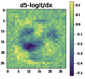
Finally we can train our model and automatically generate images when logits are “confused”

and tensorboard will automatically generate images that look like this:

Summary

In summary: You learned how to look inside the blackbox using PyTorch, learned the intuition, wrote a callback in PyTorch Lightning and automatically got your Tensorboard instance to plot questionable predictions

Try it yourself with PyTorch Lightning and PyTorch Lightning Bolts.

(This article was written ahead of an upcoming video where me (William) and Alfredo Canziani show you how to code this from scratch).

Bio: William Falcon is an AI Researcher, and Founder at PyTorch Lightning. He is trying to understand the brain, build AI and use it at scale.

Original. Reposted with permission.

Related: