 Introduction to Time Series Analysis in Python
 Introduction to Time Series Analysis in Python
Data that is updated in real-time requires additional handling and special care to prepare it for machine learning models. The important Python library, Pandas, can be used for most of this work, and this tutorial guides you through this process for analyzing time-series data.
According to Wikipedia:
A time series is a series of data points indexed (or listed or graphed) in time order. Most commonly, a time series is a sequence taken at successive equally spaced points in time. Thus it is a sequence of discrete-time data. Examples of time series are heights of ocean tides, counts of sunspots, and the daily closing value of the Dow Jones Industrial Average.
So any dataset in which is taken at successive equally spaced points in time. For example, we can see this data set that is Value of Manufacturers’ Shipments for All Manufacturing Industries.
We will see some important points that can help us in analyzing any time-series dataset. These are:
- Loading time series dataset correctly in Pandas
- Indexing in Time-Series Data
- Time-Resampling using Pandas
- Rolling Time Series
- Plotting Time-series Data using Pandas
Loading time series dataset correctly in Pandas
Let’s load the dataset mentioned above in pandas.
df = pd.read_csv('Data/UMTMVS.csv')
df.head()
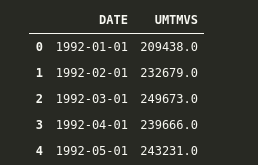
Since we want our “DATE” column as our index, but simply by reading, it is not doing it, so we have to add some extra parameters.
df = pd.read_csv(‘Data/UMTMVS.csv’, index_col=’DATE’)
df.head()
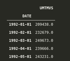
Great, now we have added our DATE column as the index, but let’s check it’s data type to know that if pandas is dealing with the index as simple objects or pandas built-in DateTime datatype.
df.index
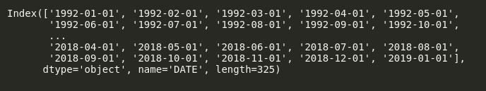
Here we can see that Pandas is dealing with our Index column as a simple object, so let’s convert it into DateTime. We can do it as follows:
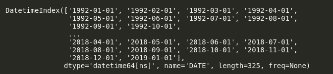
df.index = pd.to_datetime(df.index)
df.index
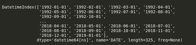
Now we can see that dtype of our dataset is datetime64[ns]. This “[ns]” shows that it is precise in nanoseconds. We can change it to “Days” or “Months” if we want.
Alternatively, to avoid all this fuss, we can load data in single line of code using Pandas as follows.
df = pd.read_csv(‘Data/UMTMVS.csv’, index_col=’DATE’, parse_dates=True)
df.index
Here we have added parse_dates=True, so it will automatically use our index as dates.
Indexing in Time-Series Data
Let’s say I want to get all the data from 2000-01-01 till 2015-05-01. In order to do this, we can simply use indexing in Pandas like this.
df.loc['2000-01-01':'2015-01-01']
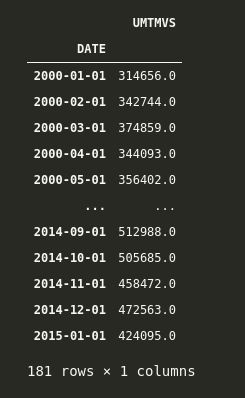
Here we have data for all the months from 2000-01-01 till 2015-01-01.
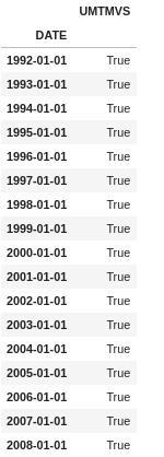
Let’s say we want to get all the data of all the first months from 1992-01-01 to 2000-01-01. We can simply do it by adding another argument that is similar to when we slice the list in python, and we add a step argument in the end.
The syntax for this in Pandas is ['starting date':'ending date':step]. Now, if we observe our dataset, it is in months format, so we want data every 12 months, from 1992 till 2000. We can do it as follows.
df.loc['1992-01-01':'2000-01-01':12]
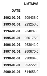
And here, we can see that we can get the values of the first month of every year.
Time-Resampling using Pandas
Think of resampling as groupby() where we group by based on any column and then apply an aggregate function to check our results. Whereas in the Time-Series index, we can resample based on any rule in which we specify whether we want to resample based on “Years” or “Months” or “Days or anything else.
Some important rules for which we resample our time series index are:
- M = Month End
- A = Year-End
- MS = Month Start
- AS = Year Start
and so on. You can check the detailed aliases in the official documentation.
Let’s apply this to our dataset.
Let’s say we want to calculate the mean value of shipment at the start of every year. We can do this by calling resample at rule='AS' for Year Start and then calling the aggregate function mean on it.
We can see the head of it as follows.
df.resample(rule='AS').mean().head()
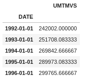
Here we have resampled the index based on starting of every year(remember what “AS” does), then applied the mean function on it, and now we have the mean of Shipping at the start of every year.
We can even use our own custom functions with resample. Let’s say we want to calculate the sum of every year with a custom function. We can do that as follows.
def sum_of_year(year_val):
    return year_val.sum()
And then we can apply it via resampling as follows.
df.resample(rule='AS').apply(year_val)
We can confirm that it is working correctly by comparing it to
df.resample(rule='AS').apply(my_own_custom) == df.resample(rule='AS').sum()
And they both are equal.
Rolling Time Series
Rolling is also similar to Time Resampling, but in Rolling, we take a window of any size and perform any function on it. In simple words, we can say that a rolling window of size k means k consecutive values.
Let’s see an example. If we want to calculate the rolling average of 10 days, we can do it as follows.
df.rolling(window=10).mean().head(20) # head to see first 20 values
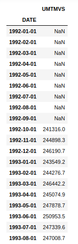
Now here, we can see that the first 10 values are NaN because there are not enough values to calculate the rolling mean for the first 10 values. It starts calculating the mean from the 11th value and goes on.
Similarly, we can check out the maximum value from a window of 30 days as follows.
df.rolling(window=30).max()[30:].head(20) # head is just to check top 20 values
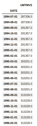
Note that here I have added [30:] just because the first 30 entries, i.e., the first window, do not have values to calculate the max function, so they are NaN, and for adding a screenshot, to show the first 20 values, I just skipped the first 30 rows, but you do not need to do it in practice.
And here, we can see that we have maximum values over a rolling window of 30 days.
Plotting Time-series Data using Pandas
Interestingly, Pandas offer a good set of built-in visualization tools and tricks which can help you in visualizing any kind of data.
A basic line plot can be obtained just by calling .plot function over the dataframe.
df.plot()
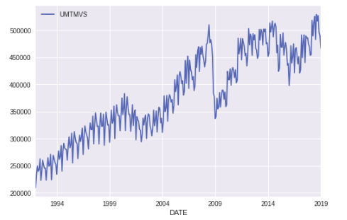
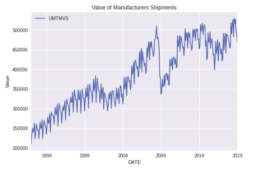
And here, we can see the value of Manufactures Shipment over time. Notice that how nicely Pandas has handled our x-axis, which is our Time Series Index.
We can further modify it by adding a title, and y-label by using .set on our plot.
ax = df.plot()
ax.set(title='Value of Manufacturers Shipments', ylabel='Value')
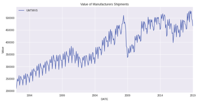
Similarly, we can change the plot size via figsize parameter in .plot.
ax = df.plot(figsize=(12,6))
ax.set(title='Value of Manufacturers Shipments', ylabel='Value')
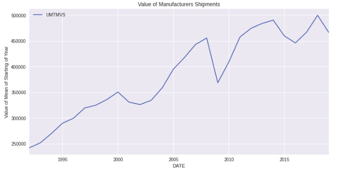
Let’s now Plot the mean of the starting value of every year. We can do it via calling .plot after resampling with the rule ‘AS’ as ‘AS’ is the rule for the starting of the year.
ax = df.resample(rule='AS').mean().plot(figsize=(12,6))
ax.set(title='Average of Manufacturers Shipments', ylabel='Value of Mean of Starting of Year')
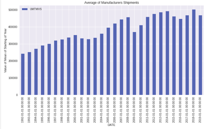
We can also do the bar plot for the mean of starting of every year by calling .bar on top of .plot.
ax = df.resample(rule='AS').mean().plot.bar(figsize=(12,6))
ax.set(title='Average of Manufacturers Shipments', ylabel='Value of Mean of Starting of Year');
Similarly, we can plot the rolling mean and normal mean for the starting of the month as follows.
ax = df['UMTMVS'].resample(rule='MS').mean().plot(figsize=(15,8), label='Resample MS')
ax.autoscale(tight=True)
df.rolling(window=30).mean()['UMTMVS'].plot(label='Rolling window=30')

ax.set(ylabel='Value of Mean of Starting of Month',title='Average of Manufacturers Shipments')
ax.legend()
Here, first, we have plotted the mean of the starting of every month via resampling on rule = “MS” (Month start). Then we have set autoscale(tight=True). This will remove the extra plot portion, which is empty. Then we have plotted the rolling mean on 30 days window. Remember that the first 30 Days are null, and you will observe this in the plot. Then we have set Label, Title, and Legend.
The output of this plot is
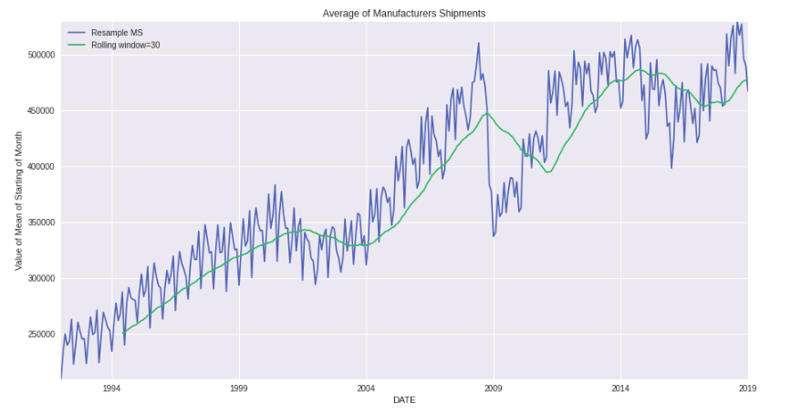
Notice how the first 30 days are missing in Rolling Average, and since it is rolling average, it is pretty smooth, as compared to resample one.
Similarly, you can plot for specific dates as per your choice. Let’s say I want to plot the maximum values for the start of every year from 1995 till 2005. I can do it as follows.
ax = df['UMTMVS'].resample(rule='AS').max().plot(xlim=["1999-01-01","2014-01-01"],ylim=[280000,540000], figsize=(12,7))
ax.yaxis.grid(True)
ax.xaxis.grid(True)
Here, we have specified the xlim and ylim. See how I have added the dates in xlim. The main pattern is xlim=['starting date', 'ending date'].
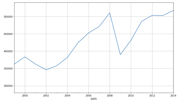
And here, you can see the output of Maximum Values at the Start of Year from 1999 till 2014.
Learning Outcomes
This brings us to the end of this article. Hopefully, you are now aware of the basics of
- Loading time series dataset correctly in Pandas
- Indexing in Time-Series Data
- Time-Resampling using Pandas
- Rolling Time Series
- Plotting Time-series Data using Pandas
these topics correctly and can apply them in your own datasets too.
Related: