The Most Complete Guide to PyTorch for Data Scientists
All the PyTorch functionality you will ever need while doing Deep Learning. From an Experimentation/Research Perspective.

PyTorch has sort of became one of the de facto standards for creating Neural Networks now, and I love its interface. Yet, it is somehow a little difficult for beginners to get a hold of.
I remember picking PyTorch up only after some extensive experimentation a couple of years back. To tell you the truth, it took me a lot of time to pick it up but am I glad that I moved from Keras to PyTorch. With its high customizability and pythonic syntax, PyTorch is just a joy to work with, and I would recommend it to anyone who wants to do some heavy lifting with Deep Learning.
So, in this PyTorch guide, I will try to ease some of the pain with PyTorch for starters and go through some of the most important classes and modules that you will require while creating any Neural Network with Pytorch.
But, that is not to say that this is aimed at beginners only as I will also talk about the high customizability PyTorch provides and will talk about custom Layers, Datasets, Dataloaders, and Loss functions.
So let’s get some coffee ☕ ️and start it up.
Tensors
Tensors are the basic building blocks in PyTorch and put very simply, they are NumPy arrays but on GPU. In this part, I will list down some of the most used operations we can use while working with Tensors. This is by no means an exhaustive list of operations you can do with Tensors, but it is helpful to understand what tensors are before going towards the more exciting parts.
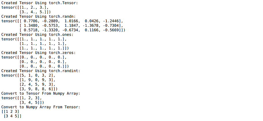
1. Create a Tensor
We can create a PyTorch tensor in multiple ways. This includes converting to tensor from a NumPy array. Below is just a small gist with some examples to start with, but you can do a whole lot of more things with tensors just like you can do with NumPy arrays.
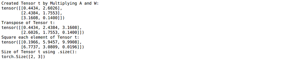
2. Tensor Operations
Again, there are a lot of operations you can do on these tensors. The full list of functions can be found here.
Note: What are PyTorch Variables? In the previous versions of Pytorch, Tensor and Variables used to be different and provided different functionality, but now the Variable API is deprecated, and all methods for variables work with Tensors. So, if you don’t know about them, it’s fine as they re not needed, and if you know them, you can forget about them.
The nn.Module

Here comes the fun part as we are now going to talk about some of the most used constructs in Pytorch while creating deep learning projects. nn.Module lets you create your Deep Learning models as a class. You can inherit from nn.Module to define any model as a class. Every model class necessarily contains an __init__ procedure block and a block for the forward pass.
- In the
__init__part, the user can define all the layers the network is going to have but doesn't yet define how those layers would be connected to each other. - In the
forwardpass block, the user defines how data flows from one layer to another inside the network.
So, put simply, any network we define will look like:
Here we have defined a very simple Network that takes an input of size 784 and passes it through two linear layers in a sequential manner. But the thing to note is that we can define any sort of calculation while defining the forward pass, and that makes PyTorch highly customizable for research purposes. For example, in our crazy experimentation mode, we might have used the below network where we arbitrarily attach our layers. Here we send back the output from the second linear layer back again to the first one after adding the input to it(skip connection) back again(I honestly don’t know what that will do).
We can also check if the neural network forward pass works. I usually do that by first creating some random input and just passing that through the network I have created.
x = torch.randn((100,784))
model = myCrazyNeuralNet()
model(x).size()
--------------------------
torch.Size([100, 10])
A word about Layers
Pytorch is pretty powerful, and you can actually create any new experimental layer by yourself using nn.Module. For example, rather than using the predefined Linear Layer nn.Linear from Pytorch above, we could have created our custom linear layer.
You can see how we wrap our weights tensor in nn.Parameter. This is done to make the tensor to be considered as a model parameter. From PyTorch docs:
Parameters are
Tensorsubclasses, that have a very special property when used withModule- when they’re assigned as Module attributes they are automatically added to the list of its parameters, and will appear inparameters()iterator
As you will later see, the model.parameters() iterator will be an input to the optimizer. But more on that later.
Right now, we can now use this custom layer in any PyTorch network, just like any other layer.
But then again, Pytorch would not be so widely used if it didn’t provide a lot of ready to made layers used very frequently in wide varieties of Neural Network architectures. Some examples are: nn.Linear, nn.Conv2d, nn.MaxPool2d, nn.ReLU, nn.BatchNorm2d, nn.Dropout, nn.Embedding, nn.GRU/nn.LSTM, nn.Softmax, nn.LogSoftmax, nn.MultiheadAttention, nn.TransformerEncoder, nn.TransformerDecoder
I have linked all the layers to their source where you could read all about them, but to show how I usually try to understand a layer and read the docs, I would try to look at a very simple convolutional layer here.
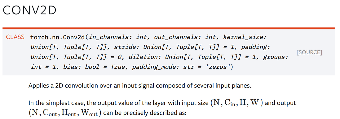
So, a Conv2d Layer needs as input an Image of height H and width W, with Cin channels. Now, for the first layer in a convnet, the number of in_channels would be 3 (RGB), and the number of out_channels can be defined by the user. The kernel_size mostly used is 3x3, and the stride normally used is 1.
To check a new layer which I don’t know much about, I usually try to see the input as well as output for the layer like below where I would first initialize the layer:
conv_layer = nn.Conv2d(in_channels = 3, out_channels = 64, kernel_size = (3,3), stride = 1, padding=1)
And then pass some random input through it. Here 100 is the batch size.
x = torch.randn((100,3,24,24))
conv_layer(x).size()
--------------------------------
torch.Size([100, 64, 24, 24])
So, we get the output from the convolution operation as required, and I have sufficient information on how to use this layer in any Neural Network I design.
Datasets and DataLoaders
How would we pass data to our Neural nets while training or while testing? We can definitely pass tensors as we have done above, but Pytorch also provides us with pre-built Datasets to make it easier for us to pass data to our neural nets. You can check out the complete list of datasets provided at torchvision.datasets and torchtext.datasets. But, to give a concrete example for datasets, let’s say we had to pass images to an Image Neural net using a folder which has images in this structure:
data
    train
        sailboat
        kayak
        .
        .
We can use torchvision.datasets.ImageFolder dataset to get an example image like below:
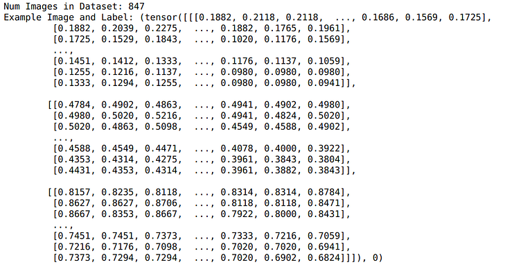
This dataset has 847 images, and we can get an image and its label using an index. Now we can pass images one by one to any image neural network using a for loop:
for i in range(0,len(train_dataset)):
    image ,label = train_dataset[i]
    pred = model(image)
But that is not optimal. We want to do batching. We can actually write some more code to append images and labels in a batch and then pass it to the Neural network. But Pytorch provides us with a utility iterator torch.utils.data.DataLoader to do precisely that. Now we can simply wrap our train_dataset in the Dataloader, and we will get batches instead of individual examples.
train_dataloader = DataLoader(train_dataset,batch_size = 64, shuffle=True, num_workers=10)
We can simply iterate with batches using:
for image_batch, label_batch in train_dataloader:
    print(image_batch.size(),label_batch.size())
    break
------------------------------------------------------------------
torch.Size([64, 3, 224, 224]) torch.Size([64])
So actually, the whole process of using datasets and Dataloaders becomes:
You can look at this particular example in action in my previous blogpost on Image classification using Deep Learning here.
This is great, and Pytorch does provide a lot of functionality out of the box. But the main power of Pytorch comes with its immense customization. We can also create our own custom datasets if the datasets provided by PyTorch don’t fit our use case.
Understanding Custom Datasets
To write our custom datasets, we can make use of the abstract class torch.utils.data.Dataset provided by Pytorch. We need to inherit this Dataset class and need to define two methods to create a custom Dataset.
__len__: a function that returns the size of the dataset. This one is pretty simple to write in most cases.__getitem__: a function that takes as input an indexiand returns the sample at indexi.
For example, we can create a simple custom dataset that returns an image and a label from a folder. See that most of the tasks are happening in __init__ part where we use glob.glob to get image names and do some general preprocessing.
Also, note that we open our images one at a time in the __getitem__ method and not while initializing. This is not done in __init__ because we don't want to load all our images in the memory and just need to load the required ones.
We can now use this dataset with the utility Dataloader just like before. It works just like the previous dataset provided by PyTorch but without some utility functions.
Understanding Custom DataLoaders
This particular section is a little advanced and can be skipped going through this post as it will not be needed in a lot of situations. But I am adding it for completeness here.
So let’s say you are looking to provide batches to a network that processes text input, and the network could take sequences with any sequence size as long as the size remains constant in the batch. For example, we can have a BiLSTM network that can process sequences of any length. It’s alright if you don’t understand the layers used in it right now; just know that it can process sequences with variable sizes.
This network expects its input to be of shape (batch_size, seq_length) and works with any seq_length. We can check this by passing our model two random batches with different sequence lengths(10 and 25).
model = BiLSTM()
input_batch_1 = torch.randint(low = 0,high = 10000, size = (100,10))
input_batch_2 = torch.randint(low = 0,high = 10000, size = (100,25))
print(model(input_batch_1).size())
print(model(input_batch_2).size())
------------------------------------------------------------------
torch.Size([100, 1])
torch.Size([100, 1])
Now, we want to provide tight batches to this model, such that each batch has the same sequence length based on the max sequence length in the batch to minimize padding. This has an added benefit of making the neural net run faster. It was, in fact, one of the methods used in the winning submission of the Quora Insincere challenge in Kaggle, where running time was of utmost importance.
So, how do we do this? Let’s write a very simple custom dataset class first.
Also, let’s generate some random data which we will use with this custom Dataset.
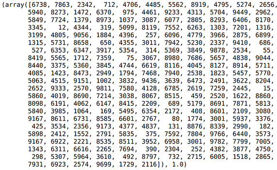
We can use the custom dataset now using:
train_dataset = CustomTextDataset(X,y)
If we now try to use the Dataloader on this dataset with batch_size>1, we will get an error. Why is that?
train_dataloader = DataLoader(train_dataset,batch_size = 64, shuffle=False, num_workers=10)
for xb,yb in train_dataloader:
    print(xb.size(),yb.size())

This happens because the sequences have different lengths, and our data loader expects our sequences of the same length. Remember that in the previous image example, we resized all images to size 224 using the transforms, so we didn’t face this error.
So, how do we iterate through this dataset so that each batch has sequences with the same length, but different batches may have different sequence lengths?
We can use collate_fn parameter in the DataLoader that lets us define how to stack sequences in a particular batch. To use this, we need to define a function that takes as input a batch and returns (x_batch, y_batch ) with padded sequence lengths based on max_sequence_length in the batch. The functions I have used in the below function are simple NumPy operations. Also, the function is properly commented so you can understand what is happening.
We can now use this collate_fn with our Dataloader as:
train_dataloader = DataLoader(train_dataset,batch_size = 64, shuffle=False, num_workers=10,collate_fn = collate_text)for xb,yb in train_dataloader:
    print(xb.size(),yb.size())
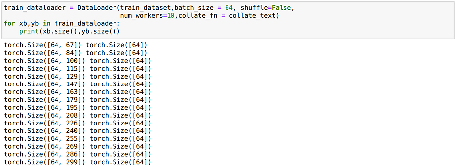
It will work this time as we have provided a custom collate_fn. And see that the batches have different sequence lengths now. Thus we would be able to train our BiLSTM using variable input sizes just like we wanted.
Training a Neural Network
We know how to create a neural network using nn.Module. But how to train it? Any neural network that has to be trained will have a training loop that will look something similar to below:
In the above code, we are running five epochs and in each epoch:
- We iterate through the dataset using a data loader.
- In each iteration, we do a forward pass using
model(x_batch) - We calculate the Loss using a
loss_criterion - We back-propagate that loss using
loss.backward()call. We don't have to worry about the calculation of the gradients at all, as this simple call does it all for us. - Take an optimizer step to change the weights in the whole network using
optimizer.step(). This is where weights of the network get modified using the gradients calculated inloss.backward()call. - We go through the validation data loader to check the validation score/metrics. Before doing validation, we set the model to eval mode using
model.eval().Please note we don't back-propagate losses in eval mode.
Till now, we have talked about how to use nn.Module to create networks and how to use Custom Datasets and Dataloaders with Pytorch. So let's talk about the various options available for Loss Functions and Optimizers.
Loss functions
Pytorch provides us with a variety of loss functions for our most common tasks, like Classification and Regression. Some most used examples are nn.CrossEntropyLoss, nn.NLLLoss, nn.KLDivLoss and nn.MSELoss. You can read the documentation of each loss function, but to explain how to use these loss functions, I will go through the example of nn.NLLLoss
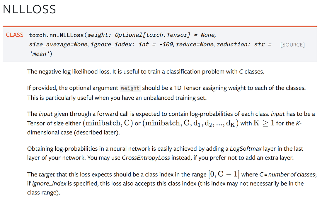
The documentation for NLLLoss is pretty succinct. As in, this loss function is used for Multiclass classification, and based on the documentation:
- the input expected needs to be of size (
batch_sizexNum_Classes) — These are the predictions from the Neural Network we have created. - We need to have the log-probabilities of each class in the input — To get log-probabilities from a Neural Network, we can add a
LogSoftmaxLayer as the last layer of our network. - The target needs to be a tensor of classes with class numbers in the range(0, C-1) where C is the number of classes.
So, we can try to use this Loss function for a simple classification network. Please note the LogSoftmax layer after the final linear layer. If you don't want to use this LogSoftmax layer, you could have just used nn.CrossEntropyLoss
Let’s define a random input to pass to our network to test it:
# some random input:X = torch.randn(100,784)
y = torch.randint(low = 0,high = 10,size = (100,))
And pass it through the model to get predictions:
model = myClassificationNet()
preds = model(X)
We can now get the loss as:
criterion = nn.NLLLoss()
loss = criterion(preds,y)
loss
------------------------------------------
tensor(2.4852, grad_fn=<NllLossBackward>)
Custom Loss Function
Defining your custom loss functions is again a piece of cake, and you should be okay as long as you use tensor operations in your loss function. For example, here is the customMseLoss
def customMseLoss(output,target):
    loss = torch.mean((output - target)**2)
    return loss
You can use this custom loss just like before. But note that we don’t instantiate the loss using criterion this time as we have defined it as a function.
output = model(x)
loss = customMseLoss(output, target)
loss.backward()
If we wanted, we could have also written it as a class using nn.Module , and then we would have been able to use it as an object. Here is an NLLLoss custom example:
Optimizers
Once we get gradients using the loss.backward() call, we need to take an optimizer step to change the weights in the whole network. Pytorch provides a variety of different ready to use optimizers using the torch.optim module. For example: torch.optim.Adadelta, torch.optim.Adagrad, torch.optim.RMSprop and the most widely used torch.optim.Adam. To use the most used Adam optimizer from PyTorch, we can simply instantiate it with:
optimizer = torch.optim.Adam(model.parameters(), lr=0.01, betas=(0.9, 0.999))
And then use optimizer.zero_grad() and optimizer.step() while training the model.
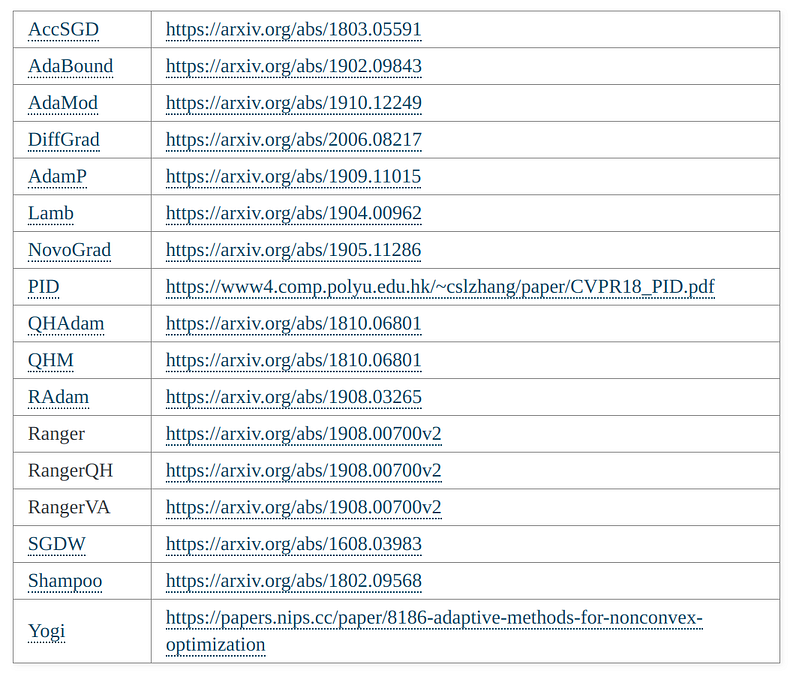
I am not discussing how to write custom optimizers as it is an infrequent use case, but if you want to have more optimizers, do check out the pytorch-optimizer library, which provides a lot of other optimizers used in research papers. Also, if you anyhow want to create your own optimizers, you can take inspiration using the source code of implemented optimizers in PyTorch or pytorch-optimizers.
Using GPU/Multiple GPUs
Till now, whatever we have done is on the CPU. If you want to use a GPU, you can put your model to GPU using model.to('cuda'). Or if you want to use multiple GPUs, you can use nn.DataParallel. Here is a utility function that checks the number of GPUs in the machine and sets up parallel training automatically using DataParallel if needed.
The only thing that we will need to change is that we will load our data to GPU while training if we have GPUs. It’s as simple as adding a few lines of code to our training loop.
Conclusion
Pytorch provides a lot of customizability with minimal code. While at first, it might be hard to understand how the whole ecosystem is structured with classes, in the end, it is simple Python. In this post, I have tried to break down most of the parts you might need while using Pytorch, and I hope it makes a little more sense for you after reading this.
You can find the code for this post here on my GitHub repo, where I keep codes for all my blogs.
If you want to learn more about Pytorch using a course based structure, take a look at the Deep Neural Networks with PyTorch course by IBM on Coursera. Also, if you want to know more about Deep Learning, I would like to recommend this excellent course on Deep Learning in Computer Vision in the Advanced machine learning specialization.
Thanks for the read. I am going to be writing more beginner-friendly posts in the future too. Follow me up at Medium or Subscribe to my blog to be informed about them. As always, I welcome feedback and constructive criticism and can be reached on Twitter @mlwhiz.
Also, a small disclaimer — There might be some affiliate links in this post to relevant resources, as sharing knowledge is never a bad idea.
Bio: Rahul Agarwal is Senior Statistical Analyst at WalmartLabs. Follow him on Twitter @mlwhiz.
Original. Reposted with permission.
Related: