 How to Evaluate the Performance of Your Machine Learning Model
 How to Evaluate the Performance of Your Machine Learning Model
You can train your supervised machine learning models all day long, but unless you evaluate its performance, you can never know if your model is useful. This detailed discussion reviews the various performance metrics you must consider, and offers intuitive explanations for what they mean and how they work.
By Saurabh Raj, IIT Jammu.
Why evaluation is necessary?
Let me start with a very simple example.
Robin and Sam both started preparing for an entrance exam for engineering college. They both shared a room and put an equal amount of hard work while solving numerical problems. They both studied almost the same hours for the entire year and appeared in the final exam. Surprisingly, Robin cleared, but Sam did not. When asked, we got to know that there was one difference in their strategy of preparation, “test series.” Robin had joined a test series, and he used to test his knowledge and understanding by giving those exams and then further evaluating where is he lagging. But Sam was confident, and he just kept training himself.
In the same fashion, as discussed above, a machine learning model can be trained extensively with many parameters and new techniques, but as long as you are skipping its evaluation, you cannot trust it.
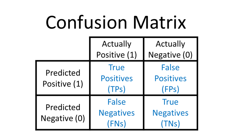
How to read the Confusion Matrix?
A confusion matrix is a correlation between the predictions of a model and the actual class labels of the data points.
Confusion Matrix for a Binary Classification.
Let’s say you are building a model that detects whether a person has diabetes or not. After the train-test split, you got a test set of length 100, out of which 70 data points are labeled positive (1), and 30 data points are labelled negative (0). Now let me draw the matrix for your test prediction:
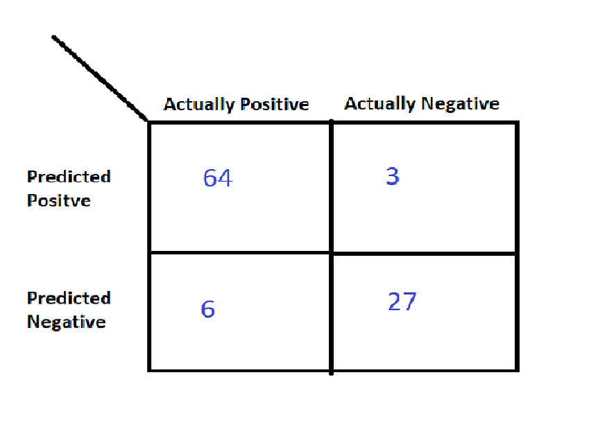
Out of 70 actual positive data points, your model predicted 64 points as positive and 6 as negative. Out of 30 actual negative points, it predicted 3 as positive and 27 as negative.
Note: In the notations, True Positive, True Negative, False Positive, & False Negative, notice that the second term (Positive or Negative) is denoting your prediction, and the first term denotes whether you predicted right or wrong.
Based on the above matrix, we can define some very important ratios:
- TPR (True Positive Rate) = ( True Positive / Actual Positive )
- TNR (True Negative Rate) = ( True Negative/ Actual Negative)
- FPR (False Positive Rate) = ( False Positive / Actual Negative )
- FNR (False Negative Rate) = ( False Negative / Actual Positive )
For our case of diabetes detection model, we can calculate these ratios:
TPR = 91.4%
TNR = 90%
FPR = 10%
FNR = 8.6%
If you want your model to be smart, then your model has to predict correctly. This means your True Positives and True Negatives should be as high as possible, and at the same time, you need to minimize your mistakes for which your False Positives and False Negatives should be as low as possible. Also in terms of ratios, your TPR & TNR should be very high whereas FPR & FNR should be very low,
A smart model: TPR ↑ , TNR ↑, FPR ↓, FNR ↓
A dumb model: Any other combination of TPR, TNR, FPR, FNR
One may argue that it is not possible to take care of all four ratios equally because, at the end of the day, no model is perfect. Then what should we do?
Yes, it is true. So that is why we build a model keeping the domain in our mind. There are certain domains that demand us to keep a specific ratio as the main priority, even at the cost of other ratios being poor. For example, in cancer diagnosis, we cannot miss any positive patient at any cost. So we are supposed to keep TPR at the maximum and FNR close to 0. Even if we predict any healthy patient as diagnosed, it is still okay as he can go for further check-ups.
Accuracy
Accuracy is what its literal meaning says, a measure of how accurate your model is.
Accuracy = Correct Predictions / Total Predictions
By using confusion matrix, Accuracy = (TP + TN)/(TP+TN+FP+FN)
Accuracy is one of the simplest performance metrics we can use. But let me warn you, accuracy can sometimes lead you to false illusions about your model, and hence you should first know your data set and algorithm used then only decide whether to use accuracy or not.
Before going to the failure cases of accuracy, let me introduce you with two types of data sets:
- Balanced:A data set that contains almost equal entries for all labels/classes. E.g., out of 1000 data points, 600 are positive, and 400 are negative.
- Imbalanced:A data set that contains a biased distribution of entries towards a particular label/class. E.g., out of 1000 entries, 990 are positive class, 10 are negative class.
Very Important: Never use accuracy as a measure when dealing with imbalanced test set.
Why?
Suppose you have an imbalanced test set of 1000 entries with 990 (+ve) and 10 (-ve). And somehow, you ended up creating a poor model which always predicts “+ve” due to the imbalanced train set. Now when you predict your test set labels, it will always predict “+ve.” So out of 1000 test set points, you get 1000 “+ve” predictions. Then your accuracy would come,
990/1000 = 99%
Whoa! Amazing! You are happy to see such an awesome accuracy score.
But, you should know that your model is really poor because it always predicts “+ve” label.
Very Important: Also, we cannot compare two models that return probability scores and have the same accuracy.
There are certain models that give the probability of each data point for belonging to a particular class like that in Logistic Regression. Let us take this case:
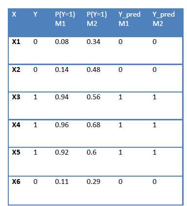
Table 1.
As you can see, If P(Y=1) > 0.5, it predicts class 1. When we calculate accuracy for both M1 and M2, it comes out the same, but it is quite evident that M1 is a much better model than M2 by taking a look at the probability scores.
This issue is beautifully dealt with by Log Loss, which I explain later in the blog.
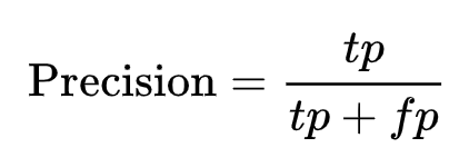
Precision & Recall
Precision: It is the ratio of True Positives (TP) and the total positive predictions. Basically, it tells us how many times your positive prediction was actually positive.
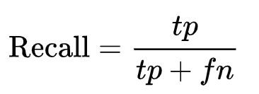
Recall : It is nothing but TPR (True Positive Rate explained above). It tells us about out of all the positive points how many were predicted positive.
F-Measure: Harmonic mean of precision and recall.
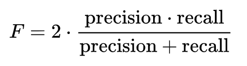
To understand this, let’s see this example: When you ask a query in google, it returns 40 pages, but only 30 were relevant. But your friend, who is an employee at Google, told you that there were 100 total relevant pages for that query. So it’s precision is 30/40 = 3/4 = 75% while it’s recall is 30/100 = 30%. So, in this case, precision is “how useful the search results are,” and recall is “how complete the results are.”
ROC & AUC
Receiver Operating Characteristic Curve (ROC):
It is a plot between TPR (True Positive Rate) and FPR (False Positive Rate) calculated by taking multiple threshold values from the reverse sorted list of probability scores given by a model.
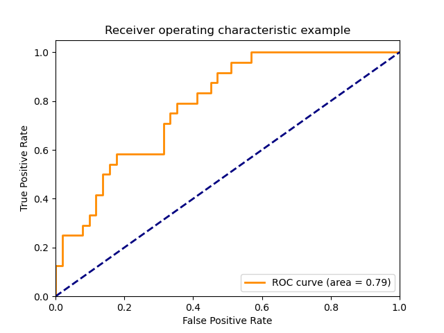
A typical ROC curve.
Now, how do we plot ROC?
To answer this, let me take you back to Table 1 above. Just consider the M1 model. You see, for all x values, we have a probability score. In that table, we have assigned the data points that have a score of more than 0.5 as class 1. Now sort all the values in descending order of probability scores and one by one take threshold values equal to all the probability scores. Then we will have threshold values = [0.96,0.94,0.92,0.14,0.11,0.08]. Corresponding to each threshold value, predict the classes, and calculate TPR and FPR. You will get 6 pairs of TPR & FPR. Just plot them, and you will get the ROC curve.
Note: Since the maximum TPR and FPR value is 1, the area under the curve (AUC) of ROC lies between 0 and 1.
The area under the blue dashed line is 0.5. AUC = 0 means very poor model, AUC = 1 means perfect model. As long as your model’s AUC score is more than 0.5. your model is making sense because even a random model can score 0.5 AUC.
Very Important: You can get very high AUC even in a case of a dumb model generated from an imbalanced data set. So always be careful while dealing with imbalanced data set.
Note: AUC had nothing to do with the numerical values probability scores as long as the order is maintained. AUC for all the models will be the same as long as all the models give the same order of data points after sorting based on probability scores.
Log Loss
This performance metric checks the deviation of probability scores of the data points from the cut-off score and assigns a penalty proportional to the deviation.
For each data point in a binary classification, we calculate it’s log loss using the formula below,
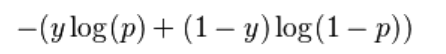
Log Loss formula for a Binary Classification.
where p = probability of the data point to belong to class 1 and y is the class label (0 or 1).
Suppose if p_1 for some x_1 is 0.95 and p_2 for some x_2 is 0.55 and cut off probability for qualifying for class 1 is 0.5. Then both qualify for class 1, but the log loss of p_2 will be much more than the log loss of p_1.
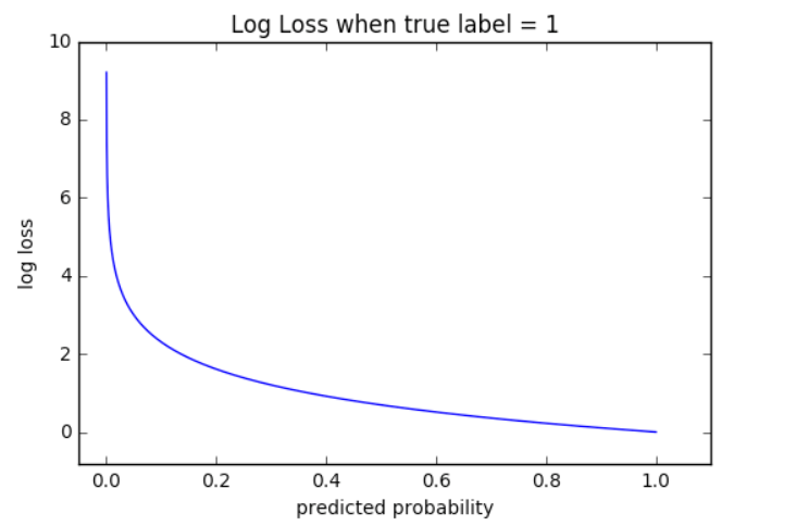
As you can see from the curve, the range of log loss is [0, infinity).
For each data point in multi-class classification, we calculate it’s log loss using the formula below,
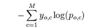
Log Loss formula for multi-class classification.
where y(o,c) = 1 if x(o,c) belongs to class 1. The rest of the concept is the same.
Coefficient of Determination
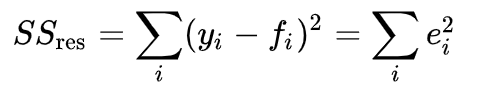
It is denoted by R². While predicting target values of the test set, we encounter a few errors (e_i), which is the difference between the predicted value and actual value.
Let’s say we have a test set with n entries. As we know, all the data points will have a target value, say [y1,y2,y3…….yn]. Let us take the predicted values of the test data be [f1,f2,f3,……fn].
Calculate the Residual Sum of Squares, which is the sum of all the errors (e_i) squared, by using this formula where fi is the predicted target value by a model for i’th data point.
Total Sum of Squares.
Take the mean of all the actual target values:
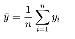
Then calculate the Total Sum of Squares, which is proportional to the variance of the test set target values:
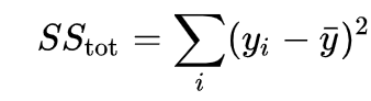
If you observe both the formulas of the sum of squares, you can see that the only difference is the 2nd term, i.e., y_bar and fi. The total sum of squares somewhat gives us an intuition that it is the same as the residual sum of squares only but with predicted values as [ȳ, ȳ, ȳ,…….ȳ ,n times]. Yes, your intuition is right. Let’s say there is a very simple mean model that gives the prediction of the average of the target values every time irrespective of the input data.
Now we formulate R² as:
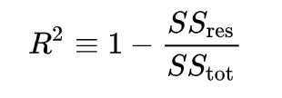
As you can see now, R² is a metric to compare your model with a very simple mean model that returns the average of the target values every time irrespective of input data. The comparison has 4 cases:
case 1: SS_R = 0
(R² = 1) Perfect model with no errors at all.
case 2: SS_R > SS_T
(R² < 0) Model is even worse than the simple mean model.
case 3: SS_R = SS_T
(R² = 0) Model is same as the simple mean model.
case 4: SS_R < SS_T
(0< R² <1) Model is okay.
Summary
So, in a nutshell, you should know your data set and problem very well, and then you can always create a confusion matrix and check for its accuracy, precision, recall, and plot the ROC curve and find out AUC as per your needs. But if your data set is imbalanced, never use accuracy as a measure. If you want to evaluate your model even more deeply so that your probability scores are also given weight, then go for Log Loss.
Remember, always evaluate your training!
Original. Reposted with permission.
Related: