Roadmap to Computer Vision
Read this introduction to the main steps which compose a computer vision system, starting from how images are pre-processed, features extracted and predictions are made.

Introduction
Computer Vision (CV) is nowadays one of the main application of Artificial Intelligence (eg. Image Recognition, Object Tracking, Multilabel Classification). In this article, I will walk you through some of the main steps which compose a Computer Vision System.
A standard representation of the workflow of a Computer Vision system is:
- A set of images enters the system.
- A Feature Extractor is used in order to pre-process and extract features from these images.
- A Machine Learning system makes use of the feature extracted in order to train a model and make predictions.
We will now briefly walk through some of the main processes our data might go through each of these three different steps.
Images Enter the System
When trying to implement a CV system, we need to take into consideration two main components: the image acquisition hardware and the image processing software. One of the main requirements to meet in order to deploy a CV system is to test its robustness. Our system should, in fact, be able to be invariant to environmental changes (such as changes in illumination, orientation, scaling) and able to perform it’s designed task repeatably. In order to satisfy these requirements, it might be necessary to apply some form of constraints to either the hardware or software of our system (eg. remotely control the lighting environment).
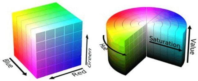
Once an image is acquired from a hardware device, there are many possible ways to numerically represents colours (Colour Spaces) within a software system. Two of the most famous colour spaces are RGB (Red, Green, Blue) and HSV (Hue, Saturation, Value). One of the main advantages of using an HSV colour space is that by taking just the HS components we can make our system illumination invariant (Figure 1).
Feature Extractor
Image Pre-processing
Once an image enters a system and is represented by using a colour space, we can then apply different operators on the image in order to improve its representation:
- Point Operators: we use all the points in an image to create a transformed version of the original image (in order to make explicit the content inside an image, without changing its content). Some examples of Point Operators are: Intensity Normalization, Histogram Equalization and Thresholding. Point Operators are commonly used in order to help visualize better an image for human vision but don’t necessarily provide any advantage for a Computer Vision system.
- Group Operators: in this case, we take a group of points from the original image in order to create a single point into the transformed version of the image. This type of operation is typically done by using Convolution. Different types of kernels can be used to be convolved with the image in order to obtain our transformed result (Figure 2). Some examples are: Direct Averaging, Gaussian Averaging and the Median Filter. Applying a convolution operation to an image can, as a result, decrease the amount of noise in the image and improve smoothing (although this can also end up slightly blurring the image). Since we are using a group of points in order to create a single new point in the new image, the dimensions of the new image will necessarily be lower than the original one. One solution to this problem is to apply either zero paddings (setting the pixel values to zero) or by using a smaller template at the border of the image. One of the main limitations of using convolution is its execution speed when working with large template sizes, one possible solution to this problem is to use a Fourier Transform instead.

Once pre-processed an image, we can then apply more advanced techniques in order to try to extract the edges and shapes within an image by using methods such as First Order Edge Detection (eg. Prewitt Operator, Sobel Operator, Canny Edge Detector) and Hough Transforms.
Feature Extraction
Once pre-processed an image, there are 4 main types of Feature Morphologies which can be extracted from an image by using a Feature Extractor:
- Global Features: the whole image is analysed as one and a single feature vector comes out of the feature extractor. A simple example of a global feature can be a histogram of binned pixel values.
- Grid or Block-Based Features: the image is split into different blocks and features are extracted from each of the different blocks. One of the main technique using in order to extract features from blocks of an image is Dense SIFT (Scale Invariant Feature Transform). This type of Features is using prevalently to train Machine Learning models.
- Region-Based Features: the image is segmented into different regions (eg. using techniques such as thresholding or K-Means Clustering and then connect them into segments using Connected Components) and a feature is extracted from each of these regions. Features can be extracted by using region and boundary description techniques such as Moments and Chain Codes).
- Local Features: multiple single interest points are detected in the image and features are extracted by analysing the pixels neighbouring the interest points. Two of the main types of interest points which can be extracted from an image are corners and blobs, these can be extracted by using methods such as the Harris & Stephens Detector and Laplacian of Gaussians. Features can finally be extracted from the detected interest points by using techniques such as SIFT (Scale Invariant Feature Transform). Local Features are typically used in order to match images to build a panorama/3D reconstruction or to retrieve images from a database.
Once extracted a set of discriminative features, we can then use them in order to train a Machine Learning model to make inference. Feature descriptors can be easily applied in Python using libraries such as OpenCV.
Machine Learning
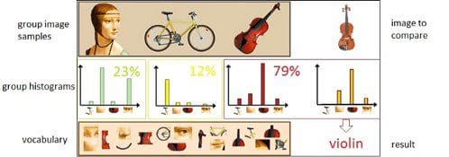
One of the main concept used in Computer Vision to classify an image is the Bag of Visual Words (BoVW). In order to construct a Bag of Visual Words, we need first of all to create a vocabulary by extracting all the features from a set of images (eg. using grid-based features or local features). Successively, we can then count the number of times an extracted feature appears in an image and build a frequency histogram from the results. Using the frequency histogram as a basic template, we can finally classify if an image belongs to the same class or not by comparing their histograms (Figure 3).
This process can be summarised in the following few steps:
- We first build a vocabulary by extracting the different features from a dataset of images using feature extraction algorithms such as SIFT and Dense SIFT.
- Secondly, we cluster all the features in our vocabulary using algorithms such as K-Means or DBSCAN and use the cluster centroids in order to summarise our data distribution.
- Finally, we can construct a frequency histogram from each image by counting the number of times different features from the vocabulary appears in the image.
New images can then be classified by repeating this same process for each image we want to classify and then using any classification algorithm to find out which image in our vocabulary resembles the most our test image.
Nowadays, thanks to the creation of Artificial Neural Networks architectures such as Convolutional Neural Networks (CNNs) and Recurrent Artificial Neural Networks (RCNNs), it has been possible to ideate an alternative workflow for Computer Vision (Figure 4).
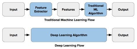
In this case, the Deep Learning Algorithm incorporates both the Feature Extraction and Classification steps of the Computer Vision workflow. When using Convolutional Neural Networks, each layer of the neural network applies the different feature extraction techniques at his description (eg. Layer 1 detects edges, Layer 2 finds shapes in an image, Layer 3 segments the image, etc…) before providing the feature vectors to the dense layer classifier.
Further applications of Machine Learning in Computer Vision include areas such as Multilabel Classification and Object Recognition. In Multilabel Classification, we aim to construct a model able to correctly identify how many objects there are in an image and to what class they do belong to. In Object Recognition instead, we aim to take this concept a step further by identifying also the position of the different objects in the image.
Contacts
If you want to keep updated with my latest articles and projects follow me on Medium and subscribe to my mailing list. These are some of my contacts details:
Bibliography
[1] Modular robot used as a beach cleaner, Felippe Roza. Researchgate. Accessed at: https://www.researchgate.net/figure/RGB-left-and-HSV-right-color-spaces_fig1_310474598
[2] Bag of visual words in OpenCV, Vision & Graphics Group. Jan Kundrac. Accessed at: https://vgg.fiit.stuba.sk/2015-02/bag-of-visual-words-in-opencv/
[3] Deep Learning Vs. Traditional Computer Vision. Haritha Thilakarathne, NaadiSpeaks. Accessed at: https://naadispeaks.wordpress.com/2018/08/12/deep-learning-vs-traditional-computer-vision/
Bio: Pier Paolo Ippolito is a Data Scientist and MSc in Artificial Intelligence graduate from the University of Southampton. He has a strong interest in AI advancements and machine learning applications (such as finance and medicine). Connect with him on Linkedin.
Original. Reposted with permission.
Related:
- Roadmap to Natural Language Processing (NLP)
- Accelerated Computer Vision: A Free Course From Amazon
- Computer Vision Recipes: Best Practices and Examples