 Monte Carlo integration in Python
 Monte Carlo integration in Python
A famous Casino-inspired trick for data science, statistics, and all of science. How to do it in Python?
Disclaimer: The inspiration for this article stemmed from Georgia Tech’s Online Masters in Analytics (OMSA) program study material. I am proud to pursue this excellent Online MS program. You can also check the details here.
What is Monte Carlo integration?
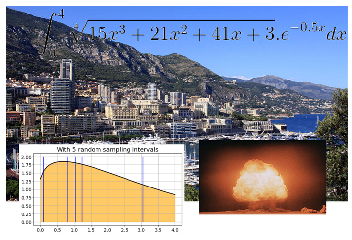
Monte Carlo, is in fact, the name of the world-famous casino located in the eponymous district of the city-state (also called a Principality) of Monaco, on the world-famous French Riviera.
It turns out that the casino inspired the minds of famous scientists to devise an intriguing mathematical technique for solving complex problems in statistics, numerical computing, system simulation.

One of the first and most famous uses of this technique was during the Manhattan Project when the chain-reaction dynamics in highly enriched uranium presented an unimaginably complex theoretical calculation to the scientists. Even the genius minds like John Von Neumann, Stanislaw Ulam, Nicholas Metropolis could not tackle it in the traditional way. They, therefore, turned to the wonderful world of random numbers and let these probabilistic quantities tame the originally intractable calculations.

Amazingly, these random variables could solve the computing problem, which stymied the sure-footed deterministic approach. The elements of uncertainty actually won.
Just like uncertainty and randomness rule in the world of Monte Carlo games. That was the inspiration for this particular moniker.

Today, it is a technique used in a wide swath of fields —
- risk analysis, financial engineering,
- supply chain logistics,
- healthcare research, drug development
- statistical learning and modeling,
- computer graphics, image processing, game design,
- large system simulations,
- computational physics, astronomy, etc.
For all its successes and fame, the basic idea is deceptively simple and easy to demonstrate. We demonstrate it in this article with a simple set of Python code.
One of the first and most famous uses of this technique was during the Manhattan Project
The idea
A tricky integral
While the general Monte Carlo simulation technique is much broader in scope, we focus particularly on the Monte Carlo integration technique here.
It is nothing but a numerical method for computing complex definite integrals, which lack closed-form analytical solutions.
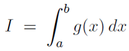
Say, we want to calculate,
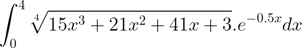
It’s not easy or downright impossible to get a closed-form solution for this integral in the indefinite form. But numerical approximation can always give us the definite integral as a sum.
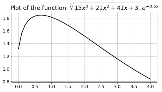
Here is the plot of the function.
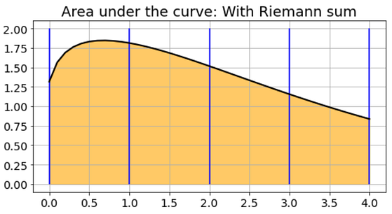
The Riemann sum
There are many such techniques under the general category of Riemann sum. The idea is just to divide the area under the curve into small rectangular or trapezoidal pieces, approximate them by the simple geometrical calculations, and sum those components up.
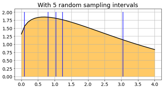
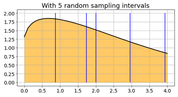
For a simple illustration, I show such a scheme with only 5 equispaced intervals.
For the programmer friends, in fact, there is a ready-made function in the Scipy package which can do this computation fast and accurately.
What if I go random?
What if I told you that I do not need to pick the intervals so uniformly, and, in fact, I can go completely probabilistic, and pick 100% random intervals to compute the same integral?
Crazy talk? My choice of samples could look like this…
Or, this…
We don’t have the time or scope to prove the theory behind it, but it can be shown that with a reasonably high number of random sampling, we can, in fact, compute the integral with sufficiently high accuracy!
We just choose random numbers (between the limits), evaluate the function at those points, add them up, and scale it by a known factor. We are done.
OK. What are we waiting for? Let’s demonstrate this claim with some simple Python code.
For all its successes and fame, the basic idea is deceptively simple and easy to demonstrate.
The Python code
Replace complex math by simple averaging
If we are trying to calculate an integral — any integral — of the form below,
we just replace the ‘estimate’ of the integral by the following average,
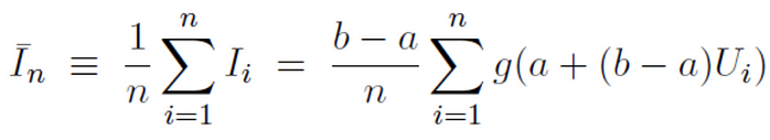
where the U’s represent uniform random numbers between 0 and 1. Note, how we replace the complex integration process by simply adding up a bunch of numbers and taking their average!
In any modern computing system, programming language, or even commercial software packages like Excel, you have access to this uniform random number generator. Check out my article on this topic,
How to generate random variables from scratch (no library used)
We go through a simple pseudo-random generator algorithm and show how to use that for generating important random…
We just choose random numbers (between the limits), evaluate the function at those points, add them up, and scale it by a known factor. We are done.
The function
Here is a Python function, which accepts another function as the first argument, two limits of integration, and an optional integer to compute the definite integral represented by the argument function.
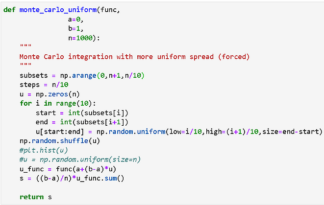
The code may look slightly different than the equation above (or another version that you might have seen in a textbook). That is because I am making the computation more accurate by distributing random samples over 10 intervals.
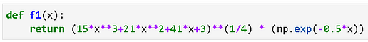
For our specific example, the argument function looks like,
And we can compute the integral by simply passing this to the monte_carlo_uniform() function,
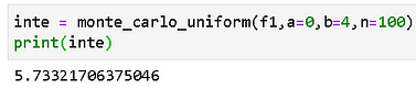
Here, as you can see, we have taken 100 random samples between the integration limits a = 0 and b = 4.
How good is the calculation anyway?
This integral cannot be calculated analytically. So, we need to benchmark the accuracy of the Monte Carlo method against another numerical integration technique anyway. We chose the Scipy integrate.quad()function for that.
Now, you may also be thinking — what happens to the accuracy as the sampling density changes. This choice clearly impacts the computation speed — we need to add less number of quantities if we choose a reduced sampling density.
Therefore, we simulated the same integral for a range of sampling density and plotted the result on top of the gold standard — the Scipy function represented as the horizontal line in the plot below,
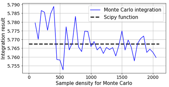
Therefore, we observe some small perturbations in the low sample density phase, but they smooth out nicely as the sample density increases. In any case, the absolute error is extremely small compared to the value returned by the Scipy function — on the order of 0.02%.
The Monte Carlo trick works fantastically!

What about the speed?
But is it as fast as the Scipy method? Better? Worse?
We try to find out by running 100 loops of 100 runs (10,000 runs in total) and obtaining the summary statistics.
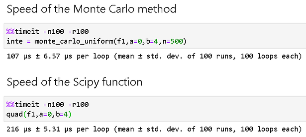
In this particular example, the Monte Carlo calculations are running twice as fast as the Scipy integration method!
While this kind of speed advantage depends on many factors, we can be assured that the Monte Carlo technique is not a slouch when it comes to the matter of computation efficiency.
we observe some small perturbations in the low sample density phase, but they smooth out nicely as the sample density increases
Rinse, repeat, rinse, and repeat…
For a probabilistic technique like Monte Carlo integration, it goes without saying that mathematicians and scientists almost never stop at just one run but repeat the calculations for a number of times and take the average.
Here is a distribution plot from a 10,000 run experiment.
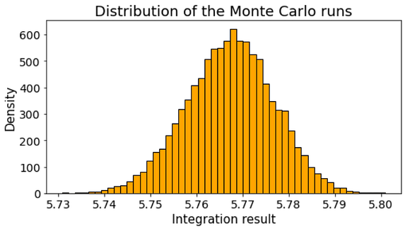
As you can see, the plot almost resembles a Gaussian Normal distribution and this fact can be utilized to not only get the average value but also construct confidence intervals around that result.
Confidence Intervals
An interval of 4 plus or minus 2 A Confidence Interval is a range of values we are fairly sure our true value lies in…
Particularly suitable for high-dimensional integrals
Although for our simple illustration (and for pedagogical purpose), we stick to a single-variable integral, the same idea can easily be extended to high-dimensional integrals with multiple variables.
And it is in this higher dimension that the Monte Carlo method particularly shines as compared to Riemann sum based approaches. The sample density can be optimized in a much more favorable manner for the Monte Carlo method to make it much faster without compromising the accuracy.
In mathematical terms, the convergence rate of the method is independent of the number of dimensions. In machine learning speak, the Monte Carlo method is the best friend you have to beat the curse of dimensionality when it comes to complex integral calculations.
Read this article for a great introduction,
Monte Carlo Methods in Practice (Monte Carlo Integration)
Monte Carlo Methods in Practice If you understand and know about the most important concepts of probability and…
And it is in this higher dimension that the Monte Carlo method particularly shines as compared to Riemann sum based approaches.
Summary
We introduced the concept of Monte Carlo integration and illustrated how it differs from the conventional numerical integration methods. We also showed a simple set of Python codes to evaluate a one-dimensional function and assess the accuracy and speed of the techniques.
The broader class of Monte Carlo simulation techniques is more exciting and is used in a ubiquitous manner in fields related to artificial intelligence, data science, and statistical modeling.
For example, the famous Alpha Go program from DeepMind used a Monte Carlo search technique to be computationally efficient in the high-dimensional space of the game Go. Numerous such examples can be found in practice.
Introduction to Monte Carlo Tree Search: The Game-Changing Algorithm behind DeepMind's AlphaGo
A best-of five-game series, $1 million dollars in prize money - A high stakes shootout. Between 9 and 15 March, 2016…
If you liked it…
If you liked this article, you may also like my other articles on similar topics,
How to generate random variables from scratch (no library used)
We go through a simple pseudo-random generator algorithm and show how to use that for generating important random…
Mathematical programming — a key habit to build up for advancing in data science
We show a small step towards building the habit of mathematical programming, a key skill in the repertoire of a budding…
Brownian motion with Python
We show how to emulate Brownian motion, the most famous stochastic process used in a wide range of applications, using…
Also, you can check the author’s GitHub repositories for code, ideas, and resources in machine learning and data science. If you are, like me, passionate about AI/machine learning/data science, please feel free to add me on LinkedIn or follow me on Twitter.
Original. Reposted with permission.
Related:
- Fast and Intuitive Statistical Modeling with Pomegranate
- The Forgotten Algorithm
- Practical Markov Chain Monte Carlo