Production Machine Learning Monitoring: Outliers, Drift, Explainers & Statistical Performance
A practical deep dive on production monitoring architectures for machine learning at scale using real-time metrics, outlier detectors, drift detectors, metrics servers and explainers.
By Alejandro Saucedo, Engineering Director at Seldon
“The lifecycle of a machine learning model only begins once it’s in production”
In this article we present an end-to-end example showcasing best practices, principles, patterns and techniques around monitoring of machine learning models in production. We will show how to adapt standard microservice monitoring techniques towards deployed machine learning models, as well as more advanced paradigms including concept drift, outlier detection and AI explainability.
We will train an image classification machine learning model from scratch, deploy it as a microservice in Kubernetes, and introduce a broad range of advanced monitoring components. The monitoring components will include outlier detectors, drift detectors, AI explainers and metrics servers — we will cover the underlying architectural patterns used for each, which are developed with scale in mind, and designed to work efficiently across hundreds or thousands of heterogeneous machine learning models.
You can also view this blog post in video form, which was presented as the keynote at the PyCon Hong Kong 2020 — the main delta is that the talk uses an Iris Sklearn model for the e2e example instead of the CIFAR10 Tensorflow model.
End to end machine learning monitoring example
In this article we present an end-to-end hands on example covering each of the high level concepts outlined in the sections below.
- Introduction to Monitoring Complex ML Systems
- CIFAR10 Tensorflow Renset32 model training
- Model Packaging & Deployment
- Performance monitoring
- Eventing Infrastructure for Monitoring
- Statistical monitoring
- Outlier detection monitoring
- Concept drift monitoring
- Explainability monitoring
We will be using the following open source frameworks in this tutorial:
- Tensorflow — Widely used machine learning framework.
- Alibi Explain — White-box and black-box ML model explanation library.
- Albi Detect — Advanced machine learning monitoring algorithms for concept drift, outlier detection and adversarial detection.
- Seldon Core — Machine learning deployment and orchestration of the models and monitoring components.
You can find the full code for this article in the jupyter notebook provided which will allow you to run all relevant steps throughout the model monitoring lifecycle.
Let’s get started.
1. Introduction to Monitoring Complex ML Systems
Monitoring of production machine learning is hard, and it becomes exponentially more complex once the number of models and advanced monitoring components grows. This is partly due to how different production machine learning systems are compared to traditional software microservice-based systems — some of these key differences are outlined below.

- Specialized hardware —Optimized implementation of machine learning algorithms often require access to GPUs, larger amounts of RAM, specialised TPUs/FPGAs, and other even dynamically changing requirements. This results in the need for specific configuration to ensure this specialised hardware can produce accurate usage metrics, and more importantly that these can be linked to the respective underlying algorithms.
- Complex Dependency Graphs — The tools and underlying data involves complex dependencies that can span across complex graph structures. This means that the processing of a single datapoint may require stateful metric assessment across multiple hops, potentially introducing additional layers of domain-specific abstraction which may have to be taken into consideration for reliable interpretation of monitoring state.
- Compliance Requirements — Production systems, especially in highly regulated environments may involve complex policies around auditing, data requirements, as well as collection of resources and artifacts at each stage of execution. Sometimes the metrics that are being displayed and analysed will have to be limited to the relevant individuals, based on the specified policies, which can vary in complexity across use-cases.
- Reproducibility — On top of these complex technical requirements, there is a critical requirement around reproducibility of components, ensuring that the components that are run can be executed at another point with the same results. When it comes to monitoring, it is important that the systems are built with this in mind such that it’s possible to re-run particular machine learning executions to reproduce particular metrics, whether for monitoring or for auditing purposes.
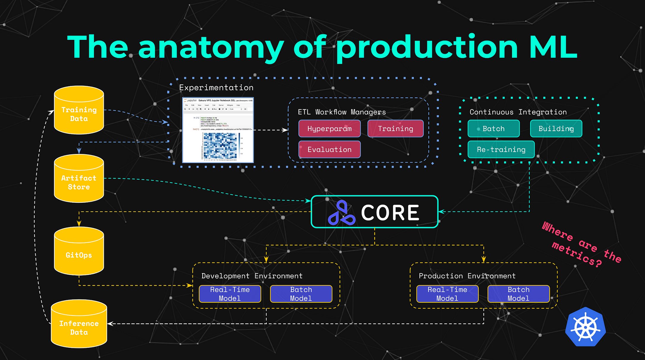
The anatomy of production machine learning involves a broad range of complexities that range across the multiple stages of the model’s lifecycle. This includes experimentation, scoring, hyperparameter tuning, serving, offline batch, streaming and beyond. Each of these stages involve potentially different systems with a broad range of heterogeneous tools. This is why it is key to ensure we not only learn how we are able to introduce model-specific metrics to monitor, but that we identify the higher level architectural patterns that can be used to enable the deployed models to be monitored effectively at scale. This is what we will cover in each of the sections below.
2. CIFAR10 Tensorflow Renset32 model training

We will be using the intuitive CIFAR10 dataset. This dataset consists of images that can be classified across one of 10 classes. The model will take as an input an array of shape 32x32x3 and as output an array with 10 probabilities for which of the classes it belongs to.
We are able to load the data from the Tensorflow datasets — namely:
The 10 classes include: cifar_classes = [“airplane”, “automobile”, “bird”, “cat”, “deer”, “dog”, “frog”, “horse”, “ship”, “truck”].
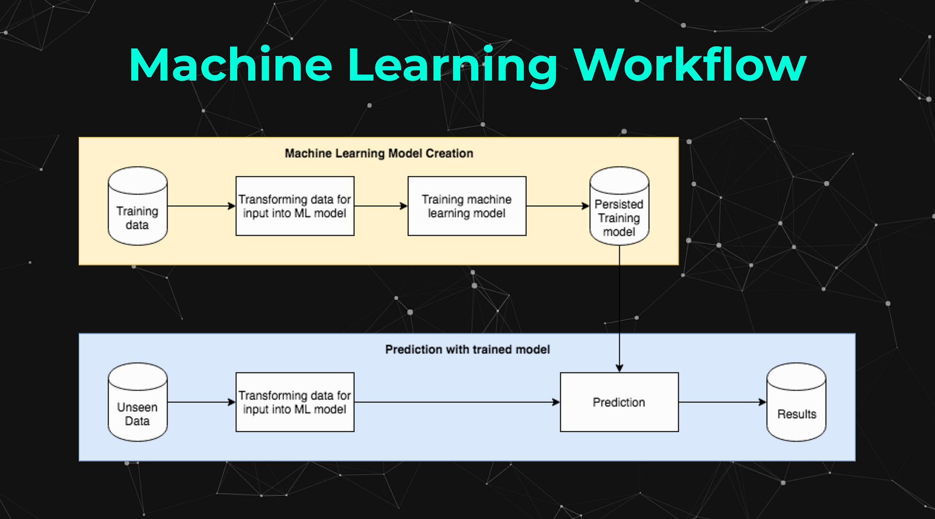
In order for us to train and deploy our machine learning model, we will follow the traditional machine learning workflow outlined in the diagram below. We will be training a model which we will then be able to export and deploy.
We will be using Tensorflow to train this model, leveraging the Residual Network which is arguably one of the most groundbreaking architectures as it makes it possible to train up to hundreds or even thousands of layers with good performance. For this tutorial we will be using the Resnet32 implementation, which fortunately we’ll be able to use through the utilities provided by the Alibi Detect Package.
Using my GPU this model took about 5 hours to train, luckily we will be able to use a pre-trained model which can be retrieved using the Alibi Detect fetch_tf_model utils.
If you want to still train the CIFAR10 resnet32 tensorflow model, you can use the helper utilities provided by the Alibi Detect package as outlined below, or even just import the raw Network and train it yourself.
We can now test the trained model on “unseen data”. We can test it using a CIFAR10 datapoint that would be classified as a truck. We can have a look at the datapoint by plotting it using Matplotlib.

We can now process that datapoint through the model, which as you can imagine should be predicted as a “truck”.
We can find the class predicted by finding the index with the highest probability, which in this case it is index 9with a high probability of 99%. From the names of the classes (e.g. cifar_classes[ np.argmax( X_curr_pred )]) we can see that class 9 is “truck”.
3. Package & deploy Model
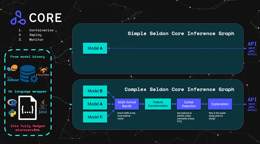
We will be using Seldon Core for the deployment of our model into Kubernetes, which provides multiple options to convert our model into a fully fledged microservice exposing REST, GRPC and Kafka interfaces.
The options we have to deploy models with Seldon Core include 1) the Language Wrappers to deploy our Python, Java, R, etc code classes, or 2) the Prepackaged Model Servers to deploy model artifacts directly. In this tutorial we will be using the Tensorflow Prepackaged Model server to deploy the Resnet32 model we were using earlier.
This approach will allow us to take advantage of the cloud native architecture of Kubernetes which powers large scale microservice systems through horizontally scalable infrastructure. We will be able to learn about and leverage cloud native and microservice patterns adopted to machine learning throughout this tutorial.
The diagram below summarises the options available to deploy model artifacts or the code itself, together with the abilities we have to deploy either a single model, or build complex inference graphs.
As a side note, you can get set up you on Kubernetes using a development environment like KIND (Kubernetes in Docker) or Minikube, and then following the instructions in the Notebook for this example, or in the Seldon documentation. You will need to make sure you install Seldon with a respective ingress provider like Istio or Ambassador so you can send the REST requests.
To simplify the tutorial, we have already uploaded the trained Tensorflow Resnet32 model, which can be found this public Google bucket: gs://seldon-models/tfserving/cifar10/resnet32. If you have trained your model, you are able to upload it to the bucket of your choice, which can be Google Bucket, Azure, S3 or local Minio. Specifically for Google you can do it using the gsutil command line with the command below:
We can deploy our model with Seldon using the custom resource definition configuration file. Below is the script that converts the model artifact into a fully fledged microservice.
We can now see that the model has been deployed and is currently running.
$ kubectl get pods | grep cifarcifar10-default-0-resnet32-6dc5f5777-sq765 2/2 Running 0 4m50sWe can now test our deployed model by sending the same image of the truck, and see if we still have the same prediction.
plt.imshow(X_curr[0])
We will be able to do this by sending a REST request as outlined below, and then print the results.
The output of the code above is the JSON response of the POST request to the url that Seldon Core provides us through the ingress. We can see that the prediction is correctly resulting in the “truck” class.
{'predictions': [[1.26448288e-06, 4.88144e-09, 1.51532642e-09, 8.49054249e-09, 5.51306611e-10, 1.16171261e-09, 5.77286274e-10, 2.88394716e-07, 0.00061489339, 0.999383569]]}

Prediction: truck
4. Performance Monitoring
The first monitoring pillar we will be covering is the good old performance monitoring, which is the traditional and standard monitoring features that you would find in the microservices and infrastructure world. Of course in our case we will be adopting it towards deployed machine learning models.
Some high level principles of machine learning monitoring include:
- Monitoring the performance of the running ML service
- Identifying potential bottlenecks or runtime red flags
- Debugging and diagnosing unexpected performance of ML services
For this we will be able to introduce the first two core frameworks which are commonly used across production systems:
- Elasticsearch for logs — A document key-value store that is commonly used to store the logs from containers, which can then be used to diagnose errors through stack traces or information logs. In the case of machine learning we don’t only use it to store logs but also to store pre-processed inputs and outputs of machine learning models for further processing.
- Prometheus for metrics —A time-series store that is commonly used to store real-time metrics data, which can then be visusalised leveraging tools like Grafana.
Seldon Core provides integration with Prometheus and Elasticsearch out of the box for any model deployed. During this tutorial we will be referencing Elasticsearch but to simplify the intuitive grasp of several advanced monitoring concepts we will be using mainly Prometheus for metrics and Grafana for the visualisations.
In the diagram below you can visualise how the exported microservice enables any containerised model to export both metrics and logs. The metrics are scraped by prometheus, and the logs are forwarded by the model into elasticsearch (which happens through the eventing infrastructure we cover in the next section. For explicitness it is worth mentioning that Seldon Core also supports Open Tracing metrics using Jaeger, which shows the latency throughout all microservice hops in the Seldon Core model graph.

Some examples of performance monitoring metrics that are exposed by Seldon Core models, and that can be also added through further integrations include:
- Requests per second
- Latency per request
- CPU/memory/data utilisation
- Custom application metrics
For this tutorial you can set up Prometheus and Grafana by using the Seldon Core Analytics package that sets everything up for metrics to be collected in real time, and then visualised on the dashboards.
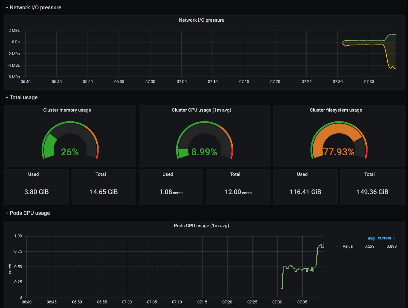
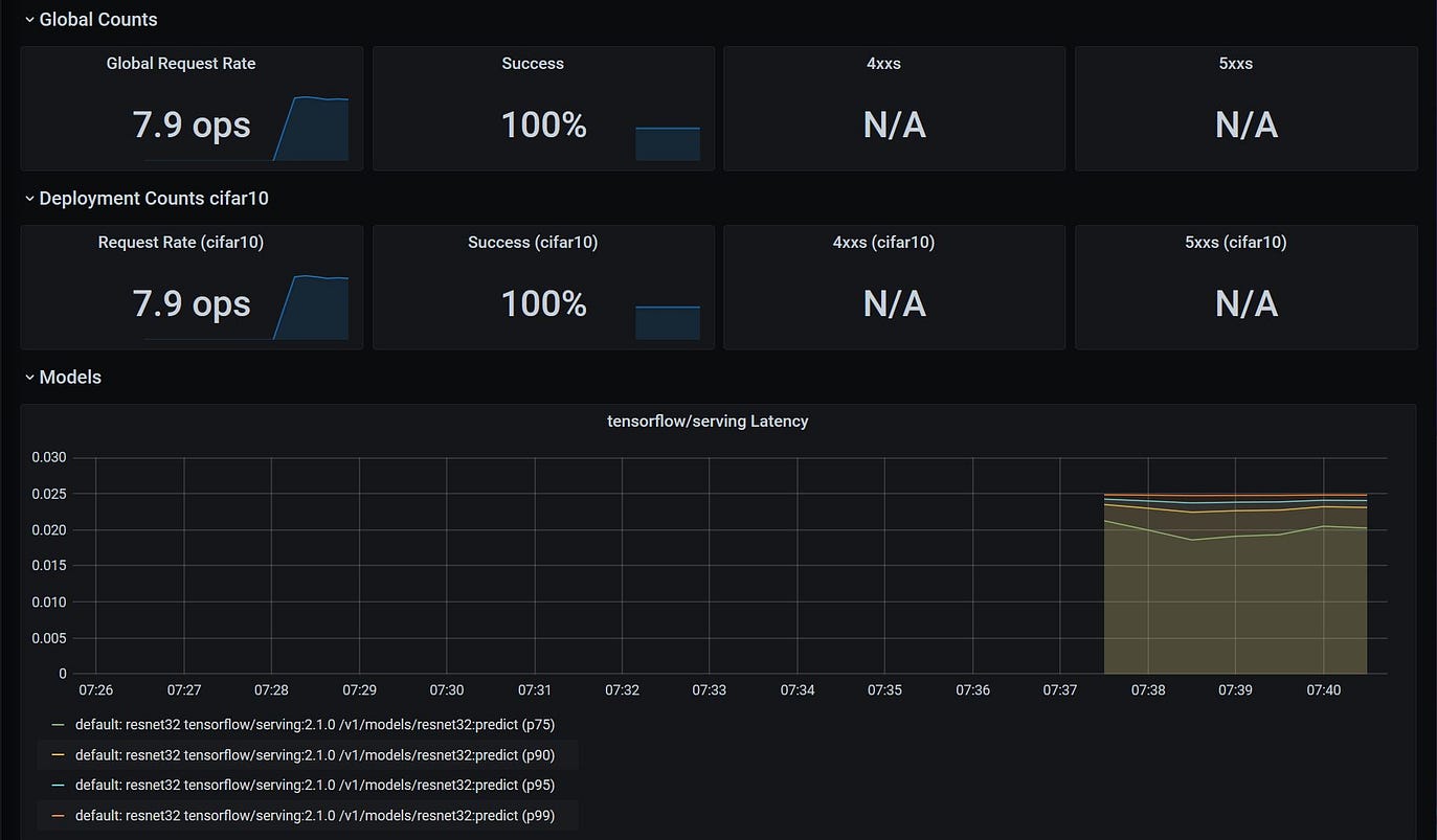
We can now visualise the utilization metrics of the deployed models relative to their specific infrastructure. When deploying a model with Seldon you will have multiple attributes that you will want to take into consideration to ensure optimal processing of your models. This includes the allocated CPU, Memory and Filesystem store reserved for the application, but also the respective configuration for running processes and threads relative to the allocated resources and expected requests.
Similarly, we are also able to monitor the usage of the model itself — every seldon model exposes model usage metrics such as requests-per-second, latency per request, success/error codes for models, etc. These are important as they are able to map into the mode advanced/specialised concepts of the underlying machine learning model. Large latency spikes could be diagnosed and explained based on the underlying requirements of the model. Similarly errors that the model displays are abstracted into simple HTTP error codes, which allows for standardisation of advanced ML components into microservice patterns that then can be managed more easily at scale by DevOps / IT managers.
5. Eventing Infrastructure for Monitoring
In order for us to be able to leverage the more advanced monitoring techniques, we will first introduce briefly the eventing infrastructure that allows Seldon to use advanced ML algorithms for monitoring of data asynchronously and in a scalable architecture.
Seldon Core leverages KNative Eventing to enable Machine Learning models to forward the inputs and outputs of the model into the more advanced machine learning monitoring components like outlier detectors, concept drift detectors, etc.
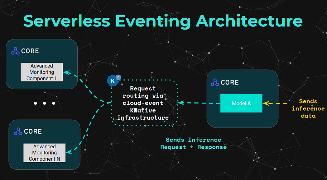
We will not be going into too much detail on the eventing infrastructure that KNative introduces, but if you are curious there are multiple hands on examples in the Seldon Core documentation in regards to how it leverages the KNative Eventing infrastructure to forward payloads to further components such as Elasticsearch, as well as how Seldon models can also be connected to process events.
For this tutorial, we need to enable our model to forward all the payload inputs and ouputs processed by the model into the KNative Eventing broker, which will enable all other advanced monitoring components to subscribe to these events.
The code below adds a “logger” attribute to the deployment configuration which specifies the broker location.
6. Statistical monitoring
Performance metrics are useful for general monitoring of microservices, however for the specialised world of machine learning, there are widely-known and widely-used metrics that are critical throughout the lifecycle of the model beyond the training phase. More common metrics can include accuracy, precision, recall, but also metrics like RMSE, KL Divergence, between many many more.
The core theme of this article is not just to specify how these metrics can be calculated, as it’s not an arduous task to enable an individual microservice to expose this through some Flask-wrapper magic. The key here is to identify scalable architectural patterns that we can introduce across hundreds or thousands of models. This means that we require a level of standardisation on the interfaces and patterns that are required to map the models into their relevant infrastructure.
Some high level principles that revolve around more specialised machine learning metrics are the following:
- Monitoring specific to statistical ML performance
- Benchmarking multiple different models or different versions
- Specialised for the data-type and the input/output format
- Stateful asynchronous provisioning of “feedback” on previous requests (such as “annotations” or “corrections”)
Given that we have these requirements, Seldon Core introduces a set of architectural patterns that allow us to introduce the concept of “Extensible Metrics Servers”. These metric servers contain out-of-the-box ways to process data that the model processes by subscribing to the respective eventing topics, to ultimately expose metrics such as:
- Raw metrics: True-Positives, True-Negatives, False-Positives, False-Negatives
- Basic metrics: Accuracy, precision, recall, specificity
- Specialised metrics: KL Divergence, RMSE, etc
- Breakdowns per class, features, and other metadata
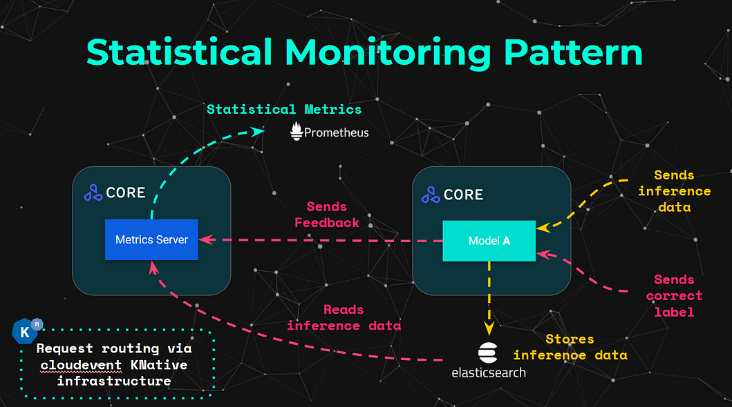
From an architectural perspective, this can be visualised more intuitively in the diagram above. This showcases how a single datapoint can be submitted through the model, and then processed by any respective Metric Servers. The metric servers can also process the “correct/annotated” labels once they are provided, which can be linked with the unique prediction ID that Seldon Core adds on every request. The specialised metrics are calculated and exposed by fetching the relevant data from the Elasticsearch store.
Currently, Seldon Core provides the following set of out-of-the-box Metrics Servers:
- BinaryClassification — Processes data in the form of binary classifications (e.g. 0 or 1) to expose raw metrics to show basic statistical metrics (accuracy, precision, recall and specificity).
- MultiClassOneHot — Processes data in the form of one hot predictions for classification tasks (e.g. [0, 0, 1] or [0, 0.2, 0.8]), which can then expose raw metrics to show basic statistical metrics.
- MultiClassNumeric — Processes data in the form of numeric datapoints for classification tasks (e.g. 1, or [1]), which can then expose raw metrics to show basic statistical metrics.
For this example we will be able to deploy a Metric Server of the type “MulticlassOneHot” — you can see the parameters used in the summarised code below, but you can find the full YAML in the jupyter notebook.
Once we deploy our metrics server, we can now just send requests and feedback to our CIFAR10 model, through the same microservice endpoint. To simplify the workflow, we will not send asynchronous feedback (which would perform the comparisons with the elasticsearch data), but instead we’ll send “self-contained” feedback requests, which contain the inference “response” and the inference “truth”.
The following function provides us with a way to send a bunch of feedback requests to achieve an approximate accuracy percent (number of correct vs incorrect predictions) for our usecase.
Now we can first send feedback to get 90% accuracy, and then to make sure our graphs look pretty, we can send another batch request that would result in 40% accuracy.
This now basically gives us the ability to visualise the metrics that the MetricsServer calculates in real time.
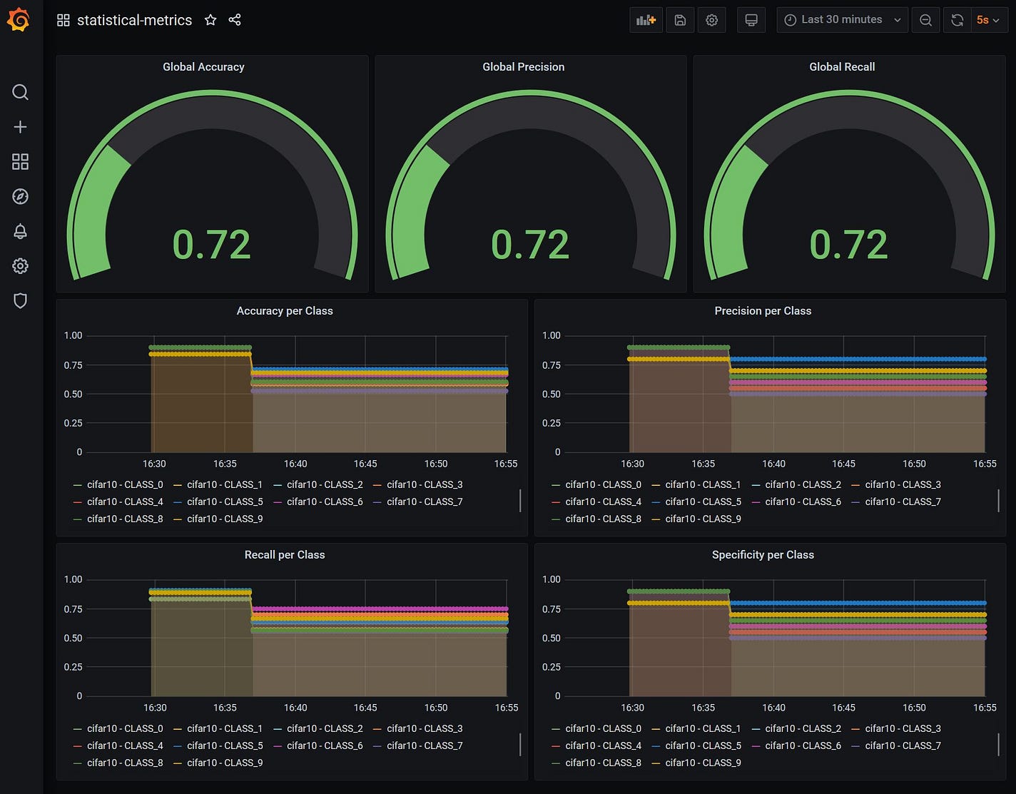
From the dashboard above we can get a high level intuition of the type of metrics that we are able to get through this architectural pattern. The stateful statistical metrics above in particular require extra metadata to be provided asynchronously, however even though the metrics themselves may have very different ways of being calculated, we can see that the infrastructural and architectural requirements can be abstracted and standardised in order for these to be approached in a more scalable way.
We will continue seeing this pattern as we delve further into the more advanced statistical monitoring techniques.
7. Outlier detection monitoring
For a more advanced monitoring technique, we will be leveraging the Alibi Detect library, particularly around some of the advanced outlier detector algorithms it provides. Seldon Core provides us with a way to perform the deployment of outlier detectors as an architectural pattern, but also provides us with a prepackaged server that is optimized to serve Alibi Detect outlier detector models.
Some of the key principles for outlier detection include:
- Detecting anomalies in data instances
- Flagging / alerting when outliers take place
- Identifying potential metadata that could help diagnose outliers
- Enable drill down of outliers that are identified
- Enabling for continuous / automated retraining of detectors
In the case of outlier detectors it is especially important to allow for the calculations to be performed separate to the model, as these tend to be much heaver and may require more specialised components. An outlier detector that is deployed, may come with similar complexities to the ones from a machine learning model, so it’s important that the same concepts of compliance, governance and lineage are covered with these advanced components.
The diagram below shows how the requests are forwarded by the model using the eventing infrastructure. The outlier detector then processes the datapoint to calculate whether it’s an outlier. The component is then able to store the outlier data in the respective request entry asynchronously, or alternatively it is able to expose the metrics to prometheus, which is what we will visualise in this section.

For this example we will be using the Alibi Detect Variational Auto Encoder outlier detector technique. The outlier detector is trained on a batch of unlabeled but normal (inlier) data. The VAE detector tries to reconstruct the input it receives, if the input data cannot be reconstructed well, then it is flagged as an outlier.
Alibi Detect provides us with utilities that allow us to export the outlier detector from scratch. We can fetch it using the fetch_detector function.
If you want to train the outlier, you can do so by simply leveraging the OutlierVAE class together with the respective encoder and decoders.
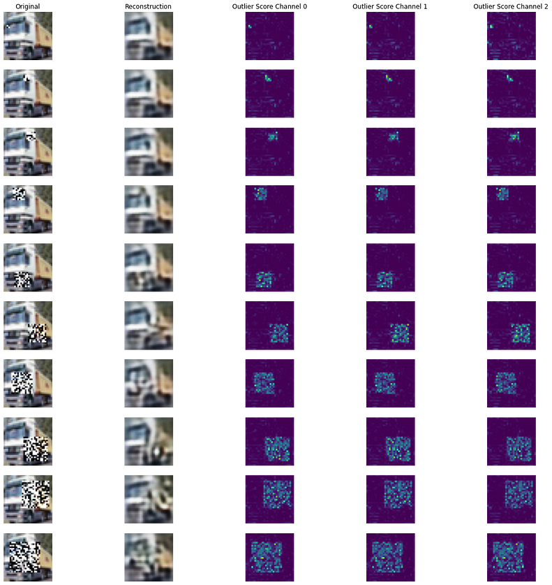
To test the outlier detector we can take the same picture of the truck and see how the outlier detector behaves if noise is added to the image increasingly. We will also be able to plot it using the Alibi Detect visualisation function plot_feature_outlier_image.
We can create a set of modified images and run it through the outlier detector using the code below.
We now have an array of modified samples in the variable all_X_mask , each with an increasing amount of noise. We can now run all these 10 through the outlier detector.
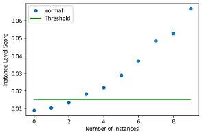
When looking at the results, we can see that the first 3 were not marked as outliers, whereas the rest were marked as outliers — we can see it by printing the value print(od_preds[“data”][“is_outlier”]). Which displays the array below, where 0 is non-outliers and 1 is outliers.
array([0, 0, 0, 1, 1, 1, 1, 1, 1, 1])We can now visualise how the outlier instance level score maps against the threshold, which reflects the results in the array above.
Similarly we can dive deeper into the intuition of what the outlier detector score channels look like, as well as the reconstructed images, which should provide a clear picture of how its internals operate.
We will now be able to productionise our outlier detector. We will be leveraging a similar architectural pattern to the one from the metric servers. Namely the Alibi Detect Seldon Core server, which will be listening to the inference input/output of the data. For every data point that goes through the model, the respective outlier detector will be able to process it.
The main step required will be to first ensure the outlier detector we trained above is uploaded to an object store like Google bucket. We have already uploaded it to gs://seldon-models/alibi-detect/od/OutlierVAE/cifar10, but if you wish you can upload it and use your own model.
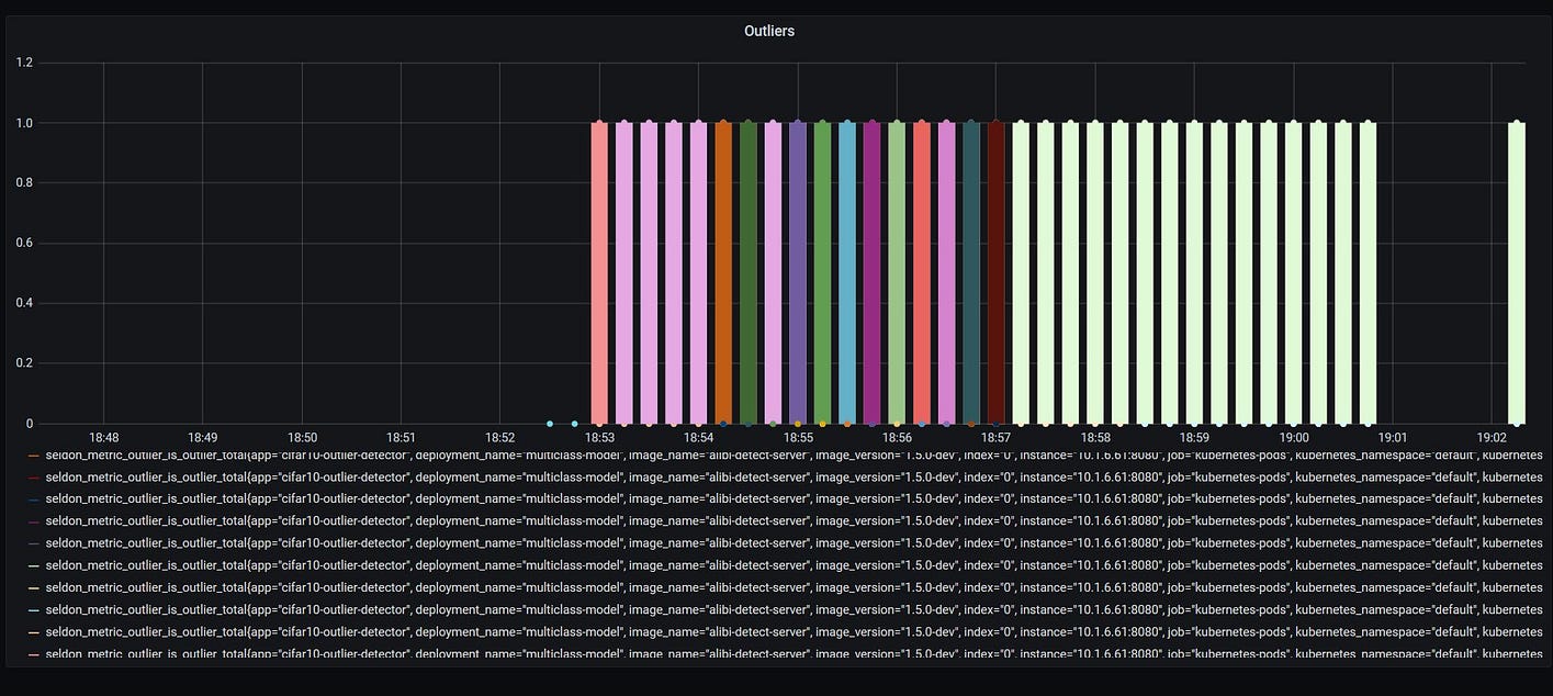
Once we deploy our outlier detector, we will be able to send a bunch of requests, many which will be outliers and others that won’t be.
We can now visualise some outliers in the dashboard — for every data point there will be a new entry point and will include whether it would be an outlier or not.
8. Drift monitoring
As time passes, data in real life production environments can change. Whilst this change is not drastic, it can be identified through drifts in the distribution of the data itself particularly in respect to the predicted outputs of the model.
Key principles in drift detection include:
- Identifying drift in data distribution, as well as drifts in the relationship between input and output data from a model
- Flagging drift that is found together with the relevant datapoints where it was identified
- Allowing for the ability to drill down into the data that was used to calculate the drift
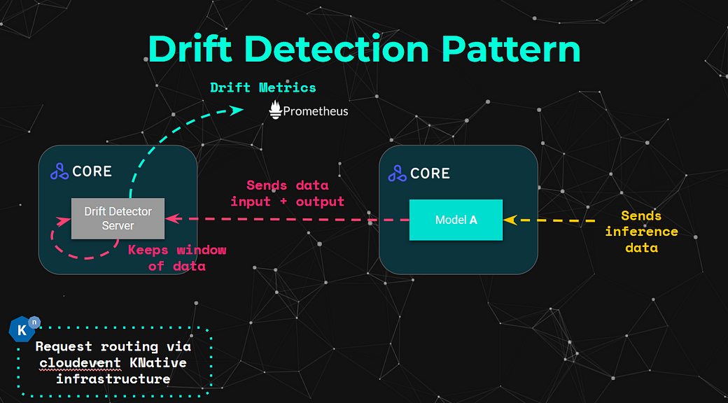
In the concept of drift detection we deal with further complexities when compared to the outlier detection usecase. The main one being the requirement to run each drift prediction on a batch input as opposed to a single datapoint. The diagram below shows a similar workflow to the one outlied in the outlier detector pattern, the main difference is that it keeps a tumbling or sliding window of data to perform the processing against.
For this example we will once again be using the Alibi Detect library, which provides us with the Kolmogorov-Smirnov data drift detector on CIFAR-10.
For this technique will be able to use the KSDrift class to create and train the drift detector, which also requires a preprocessing step which uses an “Untrained Autoencoder (UAE)”.
In order for us to test the outlier detector we will generate a set of detectors with corrupted data. Alibi Detect provides a great set of utilities that we can use to generate corruption/noise into images in an increasing way. In this case we will be using the following noise: [‘gaussian_noise’, ‘motion_blur’, ‘brightness’, ‘pixelate’]. These will be generated with the code below.
Below is one datapoint from the created corrupted dataset, which contains images with an increasing amount of corruption of the different types outlined above.

We can now attempt to run a couple of datapoints to compute whether drift is detected or not. The initial batch will consist of datapoints from the original dataset.
This as expected outputs: Drift? No!
Similarly we can run it against the corrupted dataset.
And we can see that all of them are marked as drift as expected:
Corruption type: gaussian_noise
Drift? Yes!

Corruption type: motion_blur
Drift? Yes!

Corruption type: brightness
Drift? Yes!

Corruption type: pixelate
Drift? Yes!
Deploy Drift Detector
Now we can move towards deploying our drift detector following the architectural pattern provided above. Similar to the outlier detector we first have to make sure that the drift detector we trained above can be uploaded to an object store. We currently will be able to use the Google bucket that we have prepared under gs://seldon-models/alibi-detect/cd/ks/drift to perform the deployment.
This will have a similar structure, the main difference is that we will also specify the desired batch size to use for the Alibi Detect server to keep as a buffer before running against the model. In this case we select a batch size of 1000.
Now that we have deployed our outlier detector, we first try sending 1000 requests from the normal dataset.
Next we can send the corrupted data, which would result in drift detected after sending the 10k datapoints.
We are able to visualise each of the different drift points detected in the Grafana dashboard.

9. Explainability monitoring
AI Explainability techniques are key to understanding the behaviour of complex black box machine learning models. There is a broad range of content that explores the different algorithmic techniques that can be used in different contexts. Our current focus in this context is to provide an intuition and a practical example of the architectural patterns that can allow for explainer components to be deployed at scale. Some key principles of model explainability include:
- Human-interpretable insights for model behaviour
- Introducing use-case-specific explainability capabilities
- Identifying key metrics such as trust scores or statistical perf. thresholds
- Enabling for use of some more complex ML techniques
There are a broad range of different techniques available around explainability, but it’s important to understand the high level themes around the different types of Explainers. These include:
- Scope (local vs global)
- Model type (black vs white box)
- Task (classification, regression, etc)
- Data type (tabular, images, text, etc)
- Insight (feature attributions, counterfactuals, influential training instances, etc)
For explainers as interfaces, these have similarities in the data flow patterns. Namely many of them require interacting with the data that the model processes, as well as the ability to interact with the model itself — for black box techniques it includes the inputs/outputs whereas for white-box techniques it includes the internals of the models themselves.
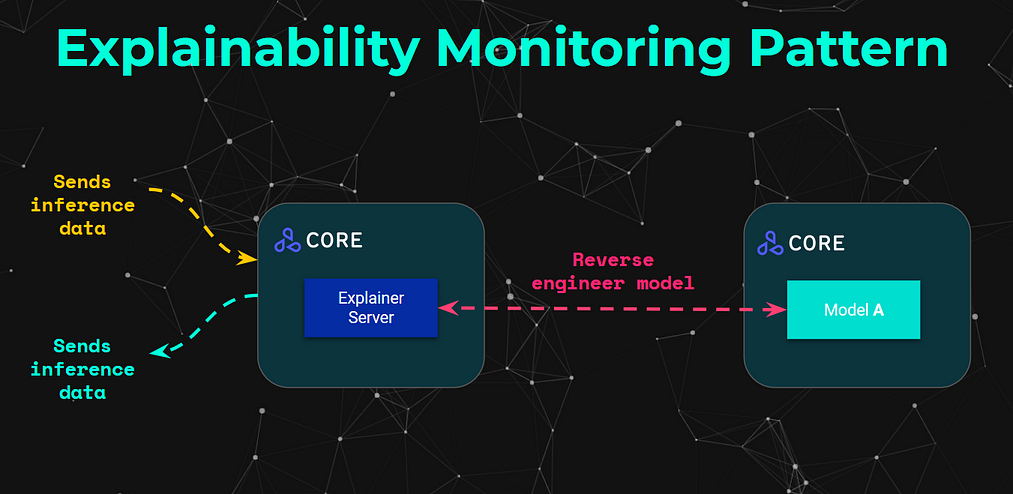
From an architectural perspective, this involves primarily a separate microservice which instead of just receiving an inference request, it would be able to interact with the respective model and “reverse engineer” the model by sending the relevant data. This is shown in the diagram above, but it will become more intuitive once we dive into the example.
For the example, we will be using the Alibi Explain framework, and we will use the Anchor Explanation technique. This local explanation technique tells us what are the features in a particular data point with the highest predictive power.
We can simply create our Anchor explainer by specifying the structure of our dataset, together with a lambda that allows the explainer to interact with the model’s predict function.
We are able to identify what are the anchors in our model that would predict in this case the image of the truck.
We can visualise the anchors by displaying the output anchor of the explanation itself.
We can see that the anchors of the image include the windshield and the wheels of the truck.

Here you can see that the explainer interacts with our deployed model. When deploying the explainer we will be following the same principle but instead of using a lambda that runs the model locally, this will be a function that will call the remote model microservice.
We will follow a similar approach where we’ll just need to upload the image above to an object store bucket. Similar to the previous example, we have provided a bucket under gs://seldon-models/tfserving/cifar10/explainer-py36–0.5.2. We will now be able to deploy an explainer, which can be deployed as part of the CRD of the Seldon Deployment.
We can check that the explainer is running with kubectl get pods | grep cifar , which should output both running pods:
cifar10-default-0-resnet32-6dc5f5777-sq765   2/2     Running   0          18m
cifar10-default-explainer-56cd6c76cd-mwjcp   1/1     Running   0          5m3s
Similar to how we send a request to the model, we are able to send a request to the explainer path. This is where the explainer will interact with the model itself and print the reverse engineered explanation.
We can see that the output of the explanation is the same as the one we saw above.
Finally we can also see some of the metric related components that come out of the explainer themselves, which can then be visualised through dashboards.
Coverage: 0.2475
Precision: 1.0
Similar to the other microservice based machine learning components deployed, the explainers also can expose these and other more specialised metrics for performance or advanced monitoring.
Closing Thoughts
Before wrapping up, one thing to outline is the importance of abstracting these advanced machine learning concepts into standardised architectural patterns. The reason why this is crucial is primarily to enable machine learning systems for scale, but also to allow for advanced integration of components across the stack.
All the advanced architectures covered above not only are applicable across each of the advanced components, but it is also possible to enable for what we can refer to as “ensemble patterns” — that is, connecting advanced components on the outputs of other advanced components.
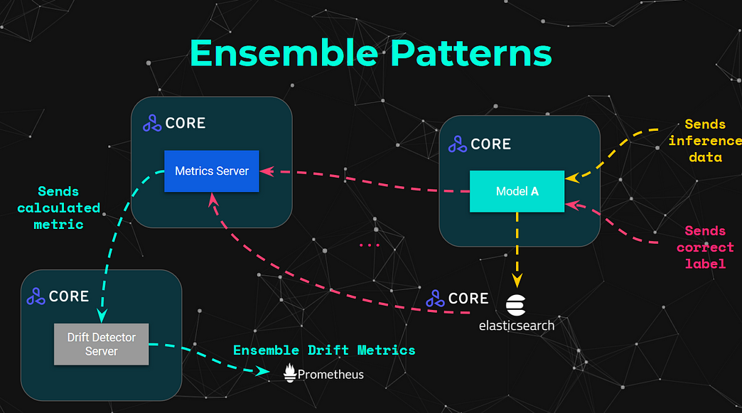
It is also important to ensure there are structured and standardised architectural patterns also enable developers to provide the monitoring components, which are also advanced machine learning models, have the same level of governance, compliance and lineage required in order to manage the risk efficiently.
These patterns are continuously being refined and evolved through the Seldon Core project, and advanced state of the art algorithms on outlier detection, concept drift, explainability, etc are improving continuously — if you are interested on furthering the discussion, please feel free to reach out. All the examples in this tutorial are open source, so suggestions are greatly appreciated.
If you are interested in further hands on examples of scalable deployment strategies of machine learning models, you can check out:
- Batch Processing with Argo Workflows
- Serverless eventing with Knative
- AI Explainability Patterns with Alibi
- Seldon Model Containerisation Notebook
- Kafka Seldon Core Stream Processing Deployment Notebook
Bio: Alejandro Saucedo is the Engineering Director at Seldon, Chief Scientist at The Institute for Ethical AI, and an ACM Council Member-at-Large.
Original. Reposted with permission.
Related:
- Interpretability, Explainability, and Machine Learning – What Data Scientists Need to Know
- Deploying Trained Models to Production with TensorFlow Serving
- AI Is More Than a Model: Four Steps to Complete Workflow Success