Photo by Markus Winkler on Unsplash.

As my knowledge in machine learning grows, so does the number of machine learning algorithms! This article will cover machine learning algorithms that are commonly used in the data science community.

Keep in mind that I’ll be elaborating on some algorithms more than others simply because this article would be as long as a book if I thoroughly explained every algorithm! I’m also going to try to minimize the amount of math in this article because I know it can be pretty daunting for those who aren’t mathematically savvy. Instead, I’ll try to give a concise summary of each and point out some of the key features.

With that in mind, I’m going to start with some of the more fundamental algorithms and then dive into some newer algorithms like CatBoost, Gradient Boost, and XGBoost.

 

Linear Regression

 

Linear Regression is one of the most fundamental algorithms used to model relationships between a dependent variable and one or more independent variables. In simpler terms, it involves finding the ‘line of best fit’ that represents two or more variables.

The line of best fit is found by minimizing the squared distances between the points and the line of best fit — this is known as minimizing the sum of squared residuals. A residual is simply equal to the predicted value minus the actual value.

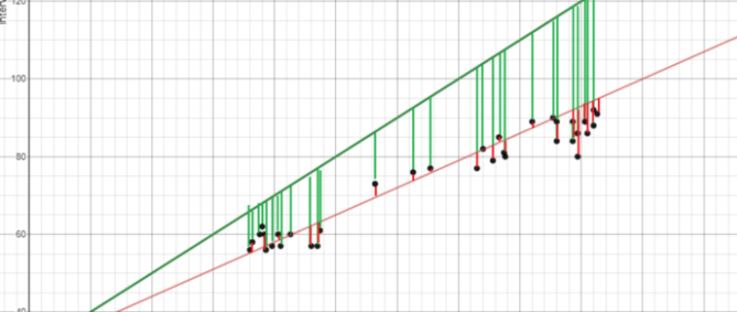
Image created by the author.

In case it doesn’t make sense yet, consider the image above. Comparing the green line of best fit to the red line, notice how the vertical lines (the residuals) are much bigger for the green line than the red line. This makes sense because the green line is so far away from the points that it isn’t a good representation of the data at all!

If you want to learn more about the math behind linear regression, I would start off with Brilliant’s explanation.

 

Logistic Regression

 

Logistic regression is similar to linear regression but is used to model the probability of a discrete number of outcomes, typically two. At a glance, logistic regression sounds much more complicated than linear regression but really only has one extra step.

First, you calculate a score using an equation similar to the equation for the line of best fit for linear regression.

The extra step is feeding the score that you previously calculated in the sigmoid function below so that you get a probability in return. This probability can then be converted to a binary output, either 1 or 0.

To find the weights of the initial equation and calculate the score, methods like gradient descent or maximum likelihood are used. Since it’s beyond the scope of this article, I won’t go into much more detail, but now you know how it works!

 

K-Nearest Neighbors

 

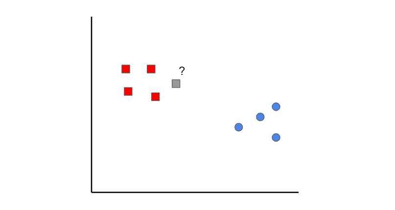
Image created by the author.

K-nearest neighbors is a simple idea. First, you start off with data that is already classified (i.e., the red and blue data points). Then when you add a new data point, you classify it by looking at the k nearest classified points. Whichever class gets the most votes determines what the new point gets classified as.

In this case, if we set k=1, we can see that the first nearest point to the grey sample is a red data point. Therefore, the point would be classified as red.

Something to keep in mind is that if the value of k is set too low, it can be subject to outliers. On the other hand, if the value of k is set too high, then it might overlook classes with only a few samples.

 

Naive Bayes

 

Naive Bayes is a classification algorithm. This means that Naive Bayes is used when the output variable is discrete.

Naive Bayes can seem like a daunting algorithm because it requires preliminary mathematical knowledge in conditional probability and Bayes Theorem, but it’s an extremely simple and ‘naive’ concept, which I’ll do my best to explain with an example:

Image created by the author.

Suppose we have input data on the characteristics of the weather (outlook, temperature, humidity, windy) and whether you played golf or not (i.e., last column).

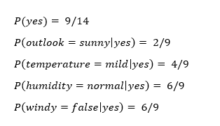
What Naive Bayes essentially does is compare the proportion between each input variable and the categories in the output variable. This can be shown in the table below.

Image created by the author.

To give an example to help you read this, in the temperature section, it was hot for two days out of the nine days that you played golf (i.e., yes).

In mathematical terms, you can write this as the probability of it being hot GIVEN that you played golf. The mathematical notation is P(hot|yes). This is known as conditional probability and is essential to understand the rest of what I’m about to say.

Once you have this, then you can predict whether you’ll play golf or not for any combination of weather characteristics.

Imagine that we have a new day with the following characteristics:

• Outlook: sunny
• Temperature: mild
• Humidity: normal
• Windy: false

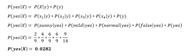
First, we’ll calculate the probability that you will play golf given X, P(yes|X), followed by the probability that you won’t play golf given X, P(no|X).

Using the chart above, we can get the following information:

Now we can simply input this information into the following formula:

Similarly, you would complete the same sequence of steps for P(no|X).

Because P(yes|X) > P(no|X), then you can predict that this person would play golf given that the outlook is sunny, the temperature is mild, the humidity is normal, and it’s not windy.

This is the essence of Naive Bayes!

 

Support Vector Machines

 

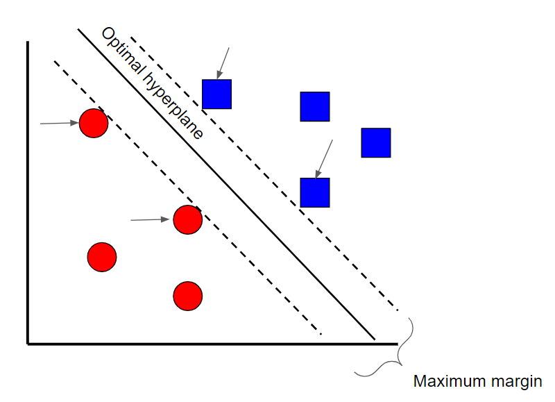
Image created by the author.

A Support Vector Machine is a supervised classification technique that can actually get pretty complicated but is pretty intuitive at the most fundamental level. For the sake of this article, we’ll keep it pretty high level.

Let’s assume that there are two classes of data. A support vector machine will find a hyperplane or a boundary between the two classes of data that maximizes the margin between the two classes (see above). There are many planes that can separate the two classes, but only one plane can maximize the margin or distance between the classes.

If you want to get into the math behind support vector machines, check out this series of articles.

Decision Tree

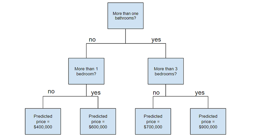
Image created by the author.

Random Forest

Before understanding random forests, there are a couple of terms that you’ll need to know:

• Ensemble learningis a method where multiple learning algorithms are used in conjunction. The purpose of doing so is that it allows you to achieve higher predictive performance than if you were to use an individual algorithm by itself.
• Bootstrap samplingis a resampling method that uses random sampling with replacement. It sounds complicated but trust me when I say it’s REALLY simple — read more about it here.
• Baggingwhen you use the aggregate of the bootstrapped datasets to make a decision — I dedicated an article to this topic, so feel free to check it out here if this doesn’t make complete sense.

Now that you understand these terms let’s dive into it.

Random forests are an ensemble learning technique that builds off of decision trees. Random forests involve creating multiple decision trees using bootstrapped datasets of the original data and randomly selecting a subset of variables at each step of the decision tree. The model then selects the mode of all of the predictions of each decision tree (bagging). What’s the point of this? By relying on a “majority wins” model, it reduces the risk of error from an individual tree.

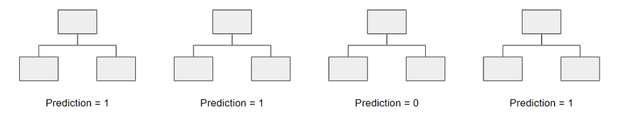
Image created by the author.

For example, if we created one decision tree, the third one, it would predict 0. But if we relied on the mode of all 4 decision trees, the predicted value would be 1. This is the power of random forests!

 

AdaBoost

 

AdaBoost, or Adaptive Boost, is also an ensemble algorithm that leverages bagging and boosting methods to develop an enhanced predictor.

AdaBoost is similar to Random Forests in the sense that the predictions are taken from many decision trees. However, there are three main differences that make AdaBoost unique:

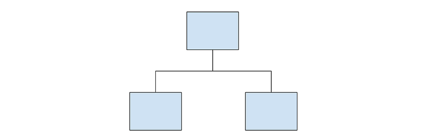
Example of a stump.

1. First, AdaBoost creates a forest of stumps rather than trees. A stump is a tree that is made of only one node and two leaves (like the image above).
2. Second, the stumps that are created are not equally weighted in the final decision (final prediction). Stumps that create more errors will have less say in the final decision.
3. Lastly, the order in which the stumps are made is important because each stump aims to reduce the errors that the previous stump(s) made.

In essence, AdaBoost takes a more iterative approach in the sense that it seeks to iteratively improve from the mistakes that the previous stump(s) made.

If you want to learn more about the underlying math behind AdaBoost, check out my article ‘A Mathematical Explanation of AdaBoost in 5 Minutes’.

 

Gradient Boost

 

It’s no surprise that Gradient Boost is also an ensemble algorithm that uses boosting methods to develop an enhanced predictor. In many ways, Gradient Boost is similar to AdaBoost, but there are a couple of key differences:

• Unlike AdaBoost, which builds stumps, Gradient Boost builds trees with usually 8–32 leaves.
• Gradient Boost views the boosting problem as an optimization problem, where it uses a loss function and tries to minimize the error. This is why it’s called Gradientboost, as it’s inspired by gradient descent.
• Lastly, the trees are used to predict the residuals of the samples (predicted minus actual).

While the last point may have been confusing, all that you need to know is that Gradient Boost starts by building one tree to try to fit the data, and the subsequent trees built after aim to reduce the residuals (error). It does this by concentrating on the areas where the existing learners performed poorly, similar to AdaBoost.

 

XGBoost

 

XGBoost is one of the most popular and widely used algorithms today because it is simply so powerful. It is similar to Gradient Boost but has a few extra features that make it that much stronger including:

• A proportional shrinking of leaf nodes (pruning) — used to improve the generalization of the model
• Newton Boosting— provides a direct route to the minima than gradient descent, making it much faster
• An extra randomization parameter — reduces the correlation between trees, ultimately improving the strength of the ensemble
• Unique penalization of trees

I strongly recommend that you watch StatQuest’s video to understand how the algorithm works in greater detail.

 

LightGBM

 

If you thought XGBoost was the best algorithm out there, think again. LightGBM is another type of boosting algorithm that has shown to be faster and sometimes more accurate than XGBoost.

What makes LightGBM different is that it uses a unique technique called Gradient-based One-Side Sampling (GOSS) to filter out the data instances to find a split value. This is different than XGBoost, which uses pre-sorted and histogram-based algorithms to find the best split.

Read more about Light GBM vs. XGBoost here!

 

CatBoost

 

CatBoost is another algorithm based on Gradient Descent that has a few subtle differences that make it unique:

• CatBoost implements symmetric trees, which help in decreasing prediction time, and it also has a shallower tree-depth by default (six)
• CatBoost leverages random permutations similar to the way XGBoost has a randomization parameter
• Unlike XGBoost however, CatBoost handles categorical features more elegantly, using concepts like ordered boosting and response coding

Overall, what makes CatBoost so powerful is its low latency requirements, which translates to it being around eight times faster than XGBoost.

If you want to read about CatBoost in greater detail, check out this article.

Thanks for Reading!

If you made it to the end, congrats! You should now have a better idea of all of the different machine learning algorithms out there.

Don’t feel discouraged if you had a harder time understanding the last few algorithms — not only are they more complex, but they’re also relatively new! So stay tuned for more resources that will go into these algorithms in greater depth.

Original. Reposted with permission.

 

Related:

• Key Data Science Algorithms Explained: From k-means to k-medoids clustering
• A Top Machine Learning Algorithm Explained: Support Vector Machines (SVM)
• Decision Tree Algorithm, Explained