Essential Math for Data Science: Introduction to Matrices and the Matrix Product

Matrices and Tensors

 
As you saw in Essential Math for Data Science, vectors are a useful way to store and manipulate data. You can represent them geometrically as arrows, or as arrays of numbers (the coordinates of their ending points). However, it can be helpful to create more complicated data structures – and that is where matrices need to be introduced.

Introduction

 
As vectors, matrices are data structures allowing you to organize numbers. They are square or rectangular arrays containing values organized in two dimensions: as rows and columns. You can think of them as a spreadsheet. Usually, you’ll see the term matrix in the context of math and two-dimensional array in the context of Numpy.

Dimensions

In the context of matrices, the term dimension is different from dimensions of the geometric representation of vectors (the dimensions of the space). When we say that a matrix is a two-dimensional array, it means that there are two directions in the array: the rows and the columns.

Matrix Notation

 
Here, I’ll denote matrices with bold typeface and upper-case letters, like A:

The matrix A has two rows and two columns but you can imagine matrices with any shape. More generally, if the matrix has m rows and n columns and contains real values, you can characterize it with the following notation: 

You can refer to matrix entries with the name of the matrix with no bold font (because the entries are scalars) followed by the index for the row and the index for the column separated by a comma in subscript. For instance, A_1,2 denotes the entry in the first row and the second column.

By convention, the first index is for the row and the second for the column. For instance, the entry 2 in the matrix A above is located in the second row and the first column of the matrix A, so it is denoted as A_2,1 (as shown in Essential Math for Data Science, one-based indexing is generally used in mathematical notation).

You can write the matrix components as follows:

Shapes

Figure 1: Matrices are two-dimensional arrays. The number of rows is usually denoted as mm and the number of columns as nn.

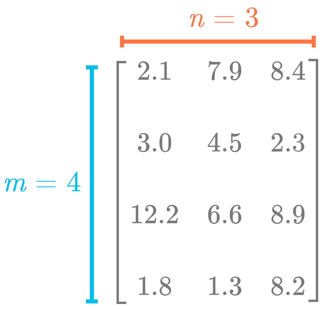
The shape of an array gives you the number of components in each dimension, as illustrated in Figure 1. Since this matrix is two-dimensional (rows and columns), you need two values to describe the shape (the number of rows and the number of columns in this order).

Let’s start by creating a 2D Numpy array with the method np.array():

A = np.array([[2.1, 7.9, 8.4],
              [3.0, 4.5, 2.3],
              [12.2, 6.6, 8.9],
              [1.8, 1., 8.2]])

Note that we use arrays in arrays ([[]]) to create the 2D array. This differs from creating a 1D array by the number of square brackets that you use.

Like with vectors, it is possible to access the shape property of Numpy arrays:

A.shape

(4, 3)

You can see that the shape contains two numbers: they correspond to the number of rows and column respectively.

Indexing

 
To get a matrix entry, you need two indexes: one to refer to the row index and one to refer to the column index.

Using Numpy, the indexing process is the same to that of vectors. You just need to specify two indexes. Let’s take again the following matrix A:

A = np.array([[2.1, 7.9, 8.4],
              [3.0, 4.5, 2.3],
              [12.2, 6.6, 8.9],
              [1.8, 1.3, 8.2]])

It is possible to get a specific entry with the following syntax:

A[1, 2]

2.3

A[1, 2] returns the component with the row index one and the column index two (with a zero-based indexing).

To get a complete column, it is possible to use a colon:

A[:, 0]

array([ 2.1,  3. , 12.2,  1.8])

This returns the first column (index zero) because the colon says that we want the components from the first to the last rows. Similarly, to get a specific row, you can do:

A[1, :]

array([3. , 4.5, 2.3])

Being able to manipulate matrices containing data is an essential skill for data scientists. Checking the shape of your data is important to be sure that it is organized the way you want. It is also important to know the data shape you’ll need to use libraries like Sklearn or Tensorflow.

Default indexing

Note that if you specify a single index from a 2D array, Numpy considers that it is for the first dimension (the rows) and all the values of the other dimension (the columns) are used. For instance

A[0]

array([2.1, 7.9, 8.4])

which is similar to:

A[0, :]

array([2.1, 7.9, 8.4])

Vectors and Matrices

With Numpy, if the array is a vector (1D Numpy array), the shape is a single number:

v = np.array([1, 2, 3])
v.shape

(3,)

You can see that v is a vector. If it is a matrix, the shape has two numbers (the number of value in the rows and in the columns respectively). For instance:

A = np.array([[2.1, 7.9, 8.4]])
A.shape

(1, 3)

You can see that the matrix has a single row: the first number of the shape is 1. Once again, using two square brackets, [[ and ]], allows you to create a two-dimensional array (a matrix).

Matrix Product

 
You learn about the dot product in Essential Math for Data Science. The equivalent operation for matrices is called the matrix product, or matrix multiplication. It takes two matrices and returns another matrix. This is a core operation in linear algebra.

Matrices with Vectors

 
The simpler case of matrix product is between a matrix and a vector (that you can consider as a matrix product with one of them having a single column).

Figure 2: Steps of the product between a matrix and a vector.

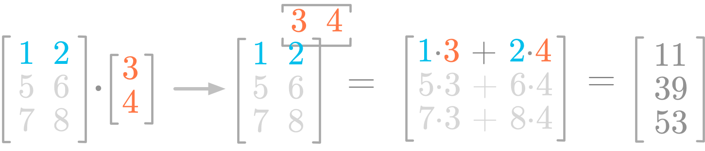
Figure 2 illustrates the steps of the product between a matrix and a vector. Let’s consider the first row of the matrix. You do the dot product between the vector (the values 3 and 4 in red) and the row you’re considering (the values 1 and 2 in blue). You multiply the values by pairs: the first value in the row with the first in the column vector (1⋅3), and the second in the row with the second in the vector (2⋅4). It gives you the first component of the resulting matrix (1⋅3+2⋅4=11).

You can see that the matrix-vector product relates to the dot product. It is like splitting the matrix AA in three rows and applying the dot product (as in Essential Math for Data Science).

Let’s see how it works with Numpy.

A = np.array([
    [1, 2],
    [5, 6],
    [7, 8]
])
v = np.array([3, 4]).reshape(-1, 1)
A @ v

array([[11],
       [39],
       [53]])

Note that we used the reshape() function to reshape the vector into a 2 by 1 matrix (the -1 tells Numpy to guess the remaining number). Without it, you would end with a one-dimensional array instead of a two-dimensional array here (a matrix with a single column).

Weighting of the Matrix’s Columns

There is another way to think about the matrix product. You can consider that the vector contains values that weight each column of the matrix. It clearly shows that the length of the vector needs to be equal to the number of columns of the matrix on which the vector is applied.

Figure 3: The vectors values are weighting the columns of the matrix.

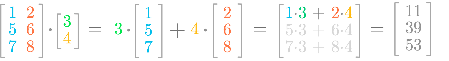
Figure 3 might help to visualize this concept. You can consider the vector values (3 and 4) as weights applied to the columns of the matrix. The rules about scalar multiplication that you saw earlier lead to the same results as before.

Using the last example, you can write the dot product between A and v as follows:

This is important because, as you’ll see in more details in Essential Math for Data Science, it shows that Av is a linear combination of the columns of A with the coefficients being the values from v.

Shapes

In addition, you can see that the shapes of the matrix and the vector must match for the dot product to be possible.

Figure 4: Shapes needed for the dot product between a matrix and a vector.

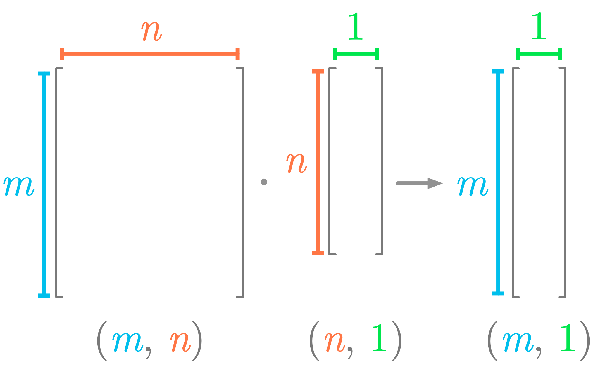
Figure 4 summarizes the shapes involved in the matrix-vector product and shows that the number of columns of the matrix must be equal to the number of rows of the vector.

Matrices Product

 
The matrix product is the equivalent of the dot product operation for two matrices. As you’ll see, it is similar to the matrix-vector product, but applied to each column of the second matrix.

Figure 5: Matrix product.

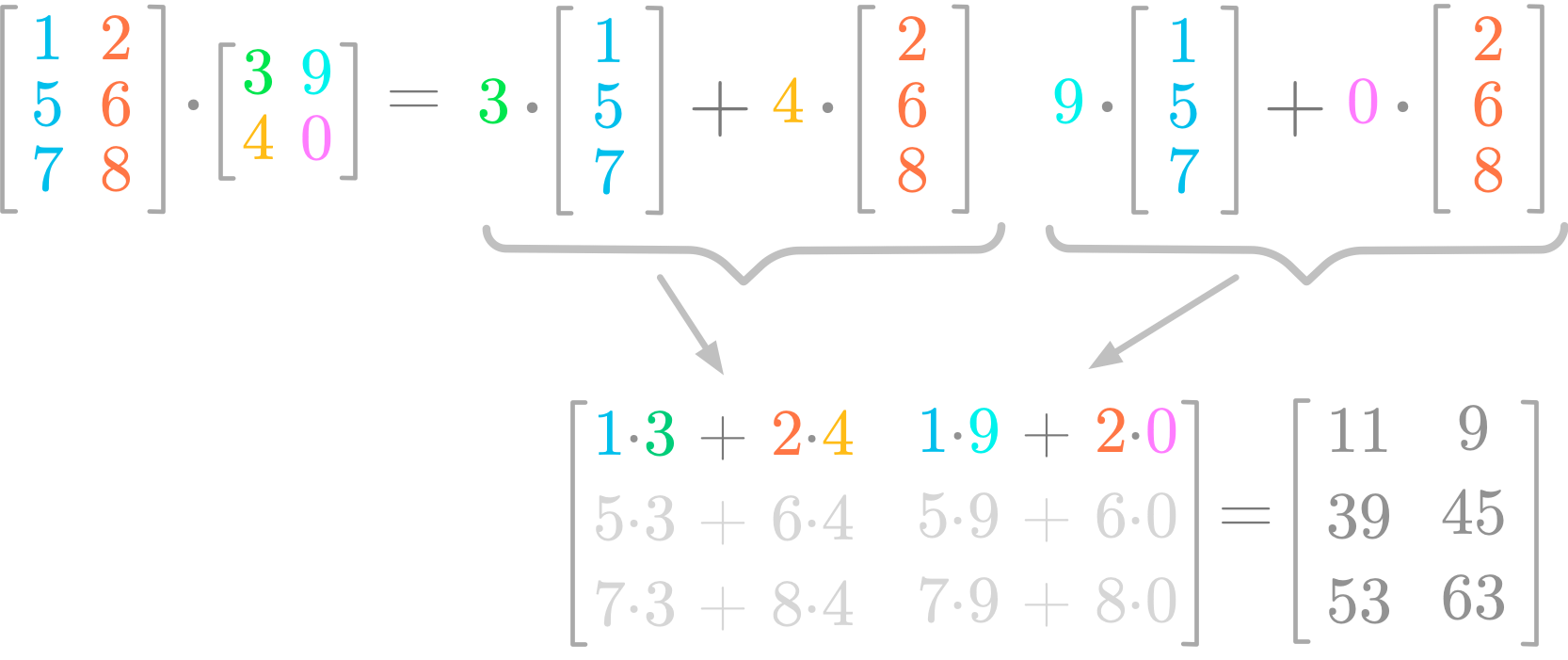
Figure 5 shows you an example of matrix product. You can see that the resulting matrix has two columns, as the second matrix. The values of first column of the second matrix (3 and 4) weight the two columns and the result fills the first column of the resulting matrix. Similarly, the values of the second column of the second matrix (9 and 0) weight the two columns and the result fills the second column of the resulting matrix.

With Numpy, you can calculate the matrix product exactly as the dot product:

A = np.array([
    [1, 2],
    [5, 6],
    [7, 8],
])
B = np.array([
    [3, 9],
    [4, 0]
])

A @ B

array([[11,  9],
       [39, 45],
       [53, 63]])

Shapes
Like with the matrix-vector product and as illustrated in Figure 6, the number of columns of the first matrix must match the number of rows of the second matrix.

Figure 6: Shapes must match for the dot product between two matrices.

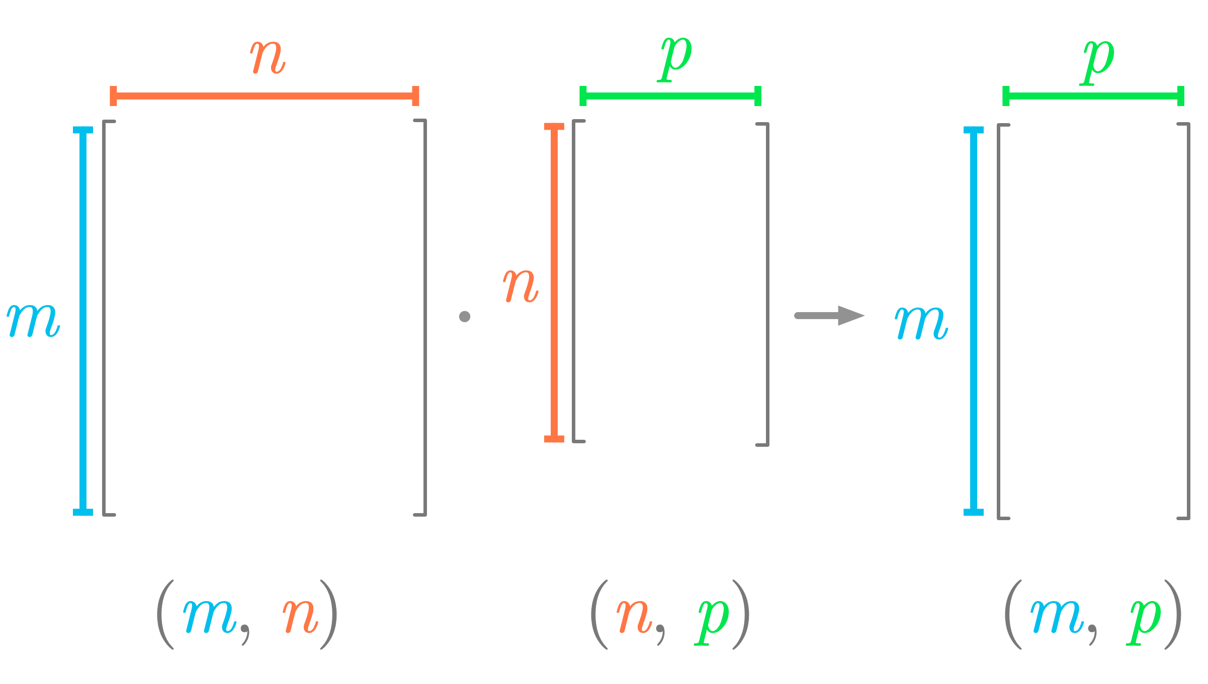
The resulting matrix has as many rows as the first matrix and as many columns as the second matrix.

Let’s try it.

A = np.array([
    [1, 4],
    [2, 5],
    [3, 6],
])

B = np.array([
    [1, 4, 7],
    [2, 5, 2],
])

The matrices A and B have different shapes. Let’s calculate their dot product:

A @ B

array([[ 9, 24, 15],
       [12, 33, 24],
       [15, 42, 33]])

You can see the result of A⋅B is a 3 by 3 matrix. This shape comes from the number of rows of A (3) and the number of columns of B (3).

Matrix Product to Calculate the Covariance Matrix

You can calculate the covariance matrix (more details about the covariance matrix in Essential Math for Data Science) of a dataset with the product between the matrix containing the variables and its transpose. Then, you divide by the number of observations (or this number minus one for the Bessel correction). You need to be sure that the variables are centered around zero beforehand (this can be done by subtracting the mean).

Let’s simulate the following variables x, y and z:

x = np.random.normal(10, 2, 100)
y = x * 1.5 + np.random.normal(25, 5, 100)
z = x * 2 + np.random.normal(0, 1, 100)

Using Numpy, the covariance matrix is:

np.cov([x, y, z])

array([[ 4.0387007 ,  4.7760502 ,  8.03240398],
       [ 4.7760502 , 32.90550824,  9.14610037],
       [ 8.03240398,  9.14610037, 16.99386265]])

Now, using the matrix product, you first need to stack the variables as columns of a matrix:

X = np.vstack([x, y, z]).T
X.shape

(100, 3)

You can see that the variable X is a 100 by 3 matrix: the 100 rows correspond to the observations and the 3 columns to the features. Then, you center this matrix around zero:

X = X - X.mean(axis=0)

Finally, you calculate the covariance matrix:

(X.T @ X) / (X.shape[0] - 1)

array([[ 4.0387007 ,  4.7760502 ,  8.03240398],
       [ 4.7760502 , 32.90550824,  9.14610037],
       [ 8.03240398,  9.14610037, 16.99386265]])

You get a covariance matrix similar to the one from the function np.cov(). This is important to keep in mind that the dot product of a matrix with its transpose corresponds to the covariance matrix.

Transpose of a Matrix Product

 
The transpose of the dot product between two matrices is defined as follows:

For instance, take the following matrices A and B:

A = np.array([
    [1, 4],
    [2, 5],
    [3, 6],
])
B = np.array([
    [1, 4, 7],
    [2, 5, 2],
])

You can check the result of  and :

(A @ B).T

array([[ 9, 12, 15],
       [24, 33, 42],
       [15, 24, 33]])

B.T @ A.T

array([[ 9, 12, 15],
       [24, 33, 42],
       [15, 24, 33]])

This can be surprising at first that the order of the two vectors or matrices in the parentheses must change for the equivalence to be satisfy. Let’s look at the details of the operation.

Figure 7: You must change the order of the vector and the matrix to obtain the transpose of the matrix product.

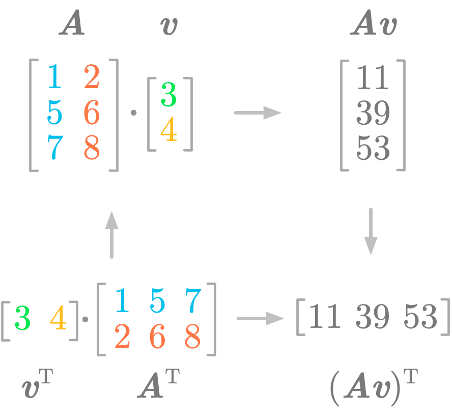
Figure 7 shows that the transpose of a matrix product is equal to the product of the transpose if you change the order of the vector and matrix.

More than two Matrices or Vectors

You can apply this property to more than two matrices or vectors. For instance,

Keep this property in a corner of your mind. It explains many “cosmetic rearrangements” that you can encounter when matrices and vectors are manipulated. Trying these manipulations with code is a great way to learn.

To conclude, the matrix product is a key concept of linear algebra, and you will see in Essential Math for Data Science how it relates to space transformation.

 
Bio: Hadrien Jean is a machine learning scientist. He owns a Ph.D in cognitive science from the Ecole Normale Superieure, Paris, where he did research on auditory perception using behavioral and electrophysiological data. He previously worked in industry where he built deep learning pipelines for speech processing. At the corner of data science and environment, he works on projects about biodiversity assessement using deep learning applied to audio recordings. He also periodically creates content and teaches at Le Wagon (data science Bootcamp), and writes articles in his blog (hadrienj.github.io).

Original. Reposted with permission.

Related:

• Essential Math for Data Science: Probability Density and Probability Mass Functions
• Matrix Decomposition Decoded
• Essential Math for Data Science: Information Theory