Machine Learning – it’s all about assumptions

By Vishal Mendekar, Skilled in Python, Machine Learning and Deep learning.

This blog is all about the assumptions made by the popular ML Algorithms, and their pros and cons.

source

Getting started with this blog, let me first tell the reason for coming up with this blog.

There are tons of Data Science enthusiasts who are either looking for a job in Data Science or switching jobs for better opportunities. Every one of these individuals must to go through some strict hiring process containing several rounds of interviews.

There are several basic questions which a recruiter/interviewer expects to be answered. Knowing about the assumptions of the popular Machine Learning Algorithms along with their Pros & Cons is one of them.

Going ahead in the blog, I will first introduce you to the assumptions made by a specific algorithm, followed by its pros & cons. So it will only take about 5 minutes of your time, and at the end of the blog, you will surely have learned something.

I am going to follow the below sequence to introduce assumption, pros & cons.

1. K-NN (K-Nearest Neighbours)
2. Logistic Regression
3. Linear Regression
4. Support Vector Machines
5. Decision Trees
6. Naive Bayes
7. Random Forest (Bagging Algorithm)
8. XGBoost (Boosting Algorithm)

 

1. K-NN

 

source

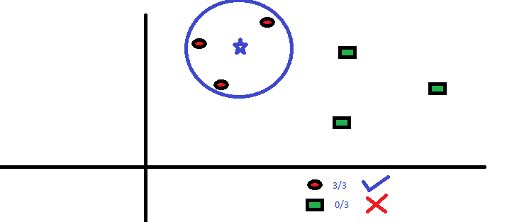
Assumptions:

1. The data is in feature space, which means data in feature space can be measured by distance metrics such as Manhattan, Euclidean, etc.
2. Each of the training data points consists of a set of vectors and a class label associated with each vector.
3. Desired to have ‘K’ as an odd number in case of 2 class classification.

Pros:

1. Easy to understand, implement, and explain.
2. Is a non-parametric algorithm, so does not have strict assumptions.
3. No training steps are required. It uses training data at run time to make predictions making it faster than all those algorithms that need to be trained.
4. Since it doesn’t need training on the train data, data points can be easily added.

Cons:

1. Inefficient and slow when the dataset is large. As for the cost of the calculation, the distance between the new point and train points is high.
2. Doesn’t work well with high dimensional data because it becomes harder to find the distance in higher dimensions.
3. Sensitive to outliers, as it is easily affected by outliers.
4. Cannot work when data is missing. So data needs to be manually imputed to make it work.
5. Needs feature scaling/normalization.

 

2. Logistic Regression

 

source

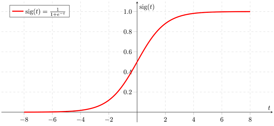
Assumptions:

1. It assumes that there is minimal or no multicollinearity among the independent variables.
2. It usually requires a large sample size to predict properly.
3. It assumes the observations to be independent of each other.

Pros:

1. Easy to interpret, implement and train. Doesn’t require too much computational power.
2. Makes no assumption of the class distribution.
3. Fast in classifying unknown records.
4. Can easily accommodate new data points.
5. Is very efficient when features are linearly separable.

Cons:

1. Tries to predict precise probabilistic outcomes, which leads to overfitting in high dimensions.
2. Since it has a linear decision surface, it can’t solve non-linear problems.
3. Tough to obtain complex relations other than linear relations.
4. Requires very little or no multicollinearity.
5. Needs a large dataset and sufficient training examples for all the categories to make correct predictions.

 

3. Linear Regression

 

source

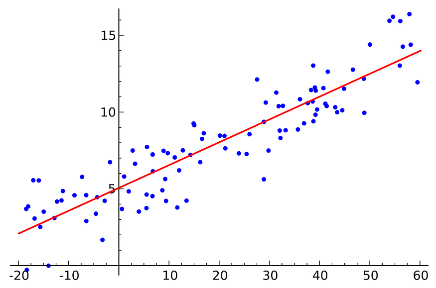
Assumptions:

1. There should be a linear relationship.
2. There should be no or little multicollinearity.
3. Homoscedasticity: The variance of residual should be the same for any value of X.

Pros:

1. Performs very well when there is a linear relationship between the independent and dependent variables.
2. If overfits, overfitting can be reduced easily by L1 or L2 Norms.

Cons:

1. Its assumption of data independence.
2. Assumption of linear separability.
3. Sensitive to outliers.

 

4. Support Vector Machines

 

source

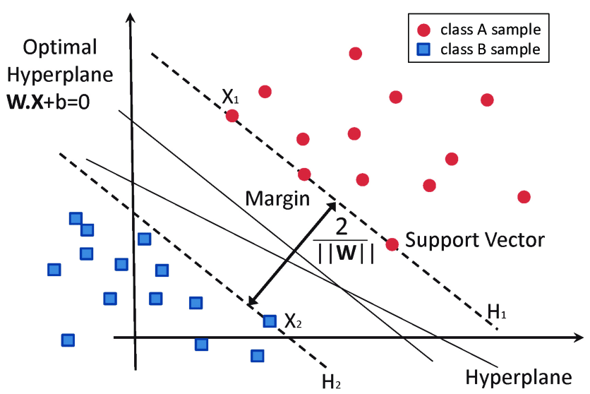
Assumptions:

1. It assumes data is independent and identically distributed.

Pros:

1. Works really well on high dimensional data.
2. Memory efficient.
3. Effective in cases where the number of dimensions is greater than the number of samples.

Cons:

1. Not suitable for large datasets.
2. Doesn’t work well when the dataset has noise, i.e., the target classes are overlapping.
3. Slow to train.
4. No probabilistic explanation for classification.

 

5. Decision Trees

 

source

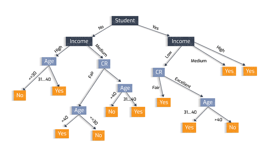
Assumptions:

1. Initially, whole training data is considered as root.
2. Records are distributed recursively on the basis of the attribute value.

Pros:

1. Compared to other algorithms, data preparation requires less time.
2. Doesn’t require data to be normalized.
3. Missing values, to an extent, don’t affect its performance much.
4. Is very intuitive as can be explained as if-else conditions.

Cons:

1. Needs a lot of time to train the model.
2. A small change in data can cause a considerably large change in the Decision Tree structure.
3. Comparatively expensive to train.
4. Not good for regression tasks.

 

6. Naive Bayes

 

source

Assumptions:

1. The biggest and only assumption is the assumption of conditional independence.

Pros:

1. Gives high performance when the conditional independence assumption is satisfied.
2. Easy to implement because only probabilities need to be calculated.
3. Works well with high-dimensional data, such as text.
4. Fast for real-time predictions.

Cons:

1. If conditional independence does not hold, then is performs poorly.
2. Has the problem of Numerical Stability or Numerical Underflow because of the multiplication of several small digits.

 

7. Random Forest

 

source

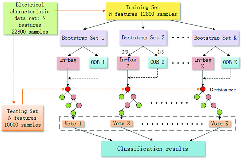
Assumptions:

1. Assumption of no formal distributions. Being a non-parametric model, it can handle skewed and multi-modal data.

Pros:

1. Robust to outliers.
2. Works well for non-linear data.
3. Low risk of overfitting.
4. Runs efficiently on large datasets.

Cons:

1. Slow training.
2. Biased when dealing with categorical variables.

 

8. XGBoost

 

source

Assumptions:

1. It may have an assumption that encoded integer value for each variable has ordinal relation.

Pros:

1. Can work in parallell.
2. Can handle missing values.
3. No need for scaling or normalizing data.
4. Fast to interpret.
5. Great execution speed.

Cons:

1. Can easily overfit if parameters are not tuned properly.
2. Hard to tune.

Original. Reposted with permission.

 

Related:

• All Machine Learning Algorithms You Should Know in 2021
• Key Data Science Algorithms Explained: From k-means to k-medoids clustering
• Know-How to Learn Machine Learning Algorithms Effectively