 Introduction to AutoEncoder and Variational AutoEncoder (VAE)
 Introduction to AutoEncoder and Variational AutoEncoder (VAE)
Autoencoders and their variants are interesting and powerful artificial neural networks used in unsupervised learning scenarios. Learn how autoencoders perform in their different approaches and how to implement with Keras on the instructional data set of the MNIST digits.

In recent years, deep learning-based generative models have gained more and more interest due to some astonishing advancements in the field of Artificial Intelligence (AI). Relying on a huge amount of data, well-designed networks architectures, and smart training techniques, deep generative models have shown an incredible ability to produce highly realistic pieces of content of various kinds, such as images, texts, and sounds.
In this article, we will dive deep into these generative networks, specifically on Autoencoders, Variational Autoencoders (VAE), and their implementation using Keras.
What is an Autoencoder?
Autoencoders (AE) are neural networks that aim to copy their inputs to their outputs. They work by compressing the input into a latent-space representation and then reconstructing the output from this representation.
An autoencoder consists of two primary components:
- Encoder: Learns to compress (reduce) the input data into an encoded representation.
- Decoder: Learns to reconstruct the original data from the encoded representation to be as close to the original input as possible.
- Bottleneck/Latent space: The layer that contains the compressed representation of the input data.
- Reconstruction loss: The method measures how well the decoder is performing, i.e., measures the difference between the encoded and decoded vectors. Lesser, the better.

The model involves encoded function g parameterized by ϕ and a decoder function f parameterized by θ. The bottleneck layer is:

the reconstructed input:

For measuring the reconstruction loss, we can use the cross-entropy (when activation function is sigmoid) or basic Mean Squared Error (MSE):

Types of vanilla autoencoders
- Undercomplete Autoencoders: An autoencoder whose latent space is less than the input dimension is called Undercomplete. Learning an undercomplete representation forces the autoencoder to capture the most salient features of the training data.
- Regularized Autoencoder: They use a loss function that encourages the model to have other properties besides the ability to copy its input to its output. In practice, we usually find two types of regularized autoencoder: the sparse autoencoder and the denoising autoencoder.
- Sparse Autoencoder: Sparse autoencoders are usually used to learn features for another task, such as classification. An autoencoder that has been regularized to be sparse must respond to unique statistical features of the dataset it has been trained on, rather than simply acting as an identity function. In this way, training to perform the copying task with a sparsity penalty can yield a model that has learned useful features as a byproduct.
- Denoising Autoencoder: The goal is no longer to reconstruct the input data. Rather than adding a penalty to the loss function, we can obtain an autoencoder that learns something useful by changing the reconstruction error term of the loss function. This can be done by adding some noise to the input image and making the autoencoder learn to remove it. By this means, the encoder will extract the most important features and learn a robust representation of the data.

Different types of Autoencoders.
Applications of Autoencoders
There are two main applications for traditional autoencoders:
- Noise removal: As we’ve seen above, Noise removal is the process of removing noise from an image. Noise reduction techniques exist for audio and images.

- Dimensionality reduction: As the encoder segment learns representations of your input data with much lower dimensionality, the encoder segments of autoencoders are useful when you wish to perform dimensionality reduction. This can especially be handy when, e.g., PCA doesn’t work, but you suspect that nonlinear dimensionality reduction does (i.e., using neural networks with nonlinear activation functions).
- Anomaly detection: By learning to replicate the most salient features in the training data under some of the constraints, the model is encouraged to learn to precisely reproduce the most frequently observed characteristics. When facing anomalies, the model should worsen its reconstruction performance. In most cases, only data with normal instances are used to train the autoencoder. After training, the autoencoder will accurately reconstruct “normal” data while failing to do so with unfamiliar anomalous data. Reconstruction error (the error between the original data and its low dimensional reconstruction) is used as an anomaly score to detect anomalies.
- Machine translation: Autoencoders have been applied to machine translation, which is usually referred to as Neural machine translation (NMT). Unlike traditional autoencoders, the output does not match the input — it is in another language. In NMT, texts are treated as sequences to be encoded into the learning procedure, while on the decoder side, sequences in the target language(s) are generated.
Dimensionality reduction in action.
Keras Implementation of Autoencoders
Let us use the famous MNIST dataset and apply autoencoders to recreate it. The MNIST dataset is comprised of 70000, 28 pixels by 28 pixels images of handwritten digits, and 70000 vectors containing information on which digit each one is.
# We create a simple AE with a single fully-connected neural layer as encoder and as decoder:

import numpy as np
import keras
from keras import layers
from keras.datasets import mnist
import matplotlib.pyplot as plt

# This is the size of our encoded representations
encoding_dim = 32  # 32 floats -> compression of factor 24.5, assuming the input is 784 floats

# This is our input image
input_img = keras.Input(shape=(784,))

# "encoded" is the encoded representation of the input
encoded = layers.Dense(encoding_dim, activation='relu')(input_img)

# "decoded" is the lossy reconstruction of the input
decoded = layers.Dense(784, activation='sigmoid')(encoded)

# This model maps an input to its reconstruction
autoencoder = keras.Model(input_img, decoded)

# Let's also create a separate encoder model:
# This model maps an input to its encoded representation
encoder = keras.Model(input_img, encoded)

# As well as the decoder model:
# This is our encoded (32-dimensional) input
encoded_input = keras.Input(shape=(encoding_dim,))

# Retrieve the last layer of the autoencoder model
decoder_layer = autoencoder.layers[-1]

# Create the decoder model
decoder = keras.Model(encoded_input, decoder_layer(encoded_input))

# Now let's train our autoencoder to reconstruct MNIST digits.
# First, we'll configure our model to use a per-pixel binary crossentropy loss, and the Adam optimizer:

autoencoder.compile(optimizer='adam', loss='binary_crossentropy')

#Let's prepare our input data. We're using MNIST digits, and we're discarding the labels (since we're only interested in encoding/decoding the input images).

(x_train, _), (x_test, _) = mnist.load_data()

# We will normalize all values between 0 and 1 and we will flatten the 28x28 images into vectors of size 784.

x_train = x_train.astype('float32') / 255.
x_test = x_test.astype('float32') / 255.
x_train = x_train.reshape((len(x_train), np.prod(x_train.shape[1:])))
x_test = x_test.reshape((len(x_test), np.prod(x_test.shape[1:])))

# Now let's train our autoencoder for 50 epochs:
autoencoder.fit(x_train, x_train,
                epochs=50,
                batch_size=256,
                shuffle=True,
                validation_data=(x_test, x_test))

# After 50 epochs, the autoencoder seems to reach a stable train/validation loss value of about 0.09. We can try to visualize the reconstructed inputs and the encoded representations. We will use Matplotlib.

# Encode and decode some digits
# Note that we take them from the *test* set

encoded_imgs = encoder.predict(x_test)
decoded_imgs = decoder.predict(encoded_imgs)
n = 10  # Number of digits to display
plt.figure(figsize=(20, 4))

for i in range(n):
    # Display original
    ax = plt.subplot(2, n, i + 1)
    plt.imshow(x_test[i].reshape(28, 28))
    plt.gray()
    ax.get_xaxis().set_visible(False)
    ax.get_yaxis().set_visible(False)

# Display reconstruction
    ax = plt.subplot(2, n, i + 1 + n)
    plt.imshow(decoded_imgs[i].reshape(28, 28))
    plt.gray()
    ax.get_xaxis().set_visible(False)
    ax.get_yaxis().set_visible(False)
plt.show()
Here’s what we get. The top row is the original digits, and the bottom row is the reconstructed digits. We are losing quite a bit of detail with this basic approach.

Limitations of Autoencoders for Content Generation
After we train an autoencoder, we might think about whether we can use the model to create new content. Particularly, we may ask can we make a point randomly from that latent space and decode it to get new content?
The answer is “yes,” but the quality and relevance of generated data depend on the regularity of the latent space. The latent space regularity depends on the distribution of the initial data, the dimension of the latent space, and the architecture of the encoder. It is quite difficult to ensure, a priori, that the encoder will organize the latent space in a smart way compatible with the generative process I mentioned. No regularization means overfitting, which leads to meaningless content once decoded for some point.
How can we make sure the latent space is regularized enough? We can explicitly introduce regularization during the training process. Therefore, we introduce Variational Autoencoders.
What is Variational Autoencoder (VAE)?
Variational autoencoder (VAE) is a slightly more modern and interesting take on autoencoding.
A VAE assumes that the source data has some sort of underlying probability distribution (such as Gaussian) and then attempts to find the parameters of the distribution. Implementing a variational autoencoder is much more challenging than implementing an autoencoder. The one main use of a variational autoencoder is to generate new data that’s related to the original source data. Now, exactly what the additional data is good for is hard to say. A variational autoencoder is a generative system and serves a similar purpose as a generative adversarial network (although GANs work quite differently).

Variational Autoencoders(VAE).
Mathematics behind Variational Autoencoder (VAE)
VAE uses KL-divergence as its loss function. The goal of this is to minimize the difference between a supposed distribution and the original distribution of a dataset.
Suppose we have a distribution z, and we want to generate the observation x from it. In other words, we want to calculate:

We can do it by following way:

But, the calculation of p(x) can be done by using integration as:

This usually makes it an intractable distribution(take equal to or more than exponential-time). Hence, we need to approximate p(z|x) to q(z|x) to make it a tractable distribution. To better approximate p(z|x) to q(z|x), we will minimize the KL-divergence loss, which calculates how similar two distributions are:

By simplifying, the above minimization problem is equivalent to the following maximization problem :

The first term represents the reconstruction likelihood, and the other term ensures that our learned distribution q is similar to the true prior distribution p.
Thus our total loss consists of two terms, one is reconstruction error, and the other is KL-divergence loss:

Keras Implementation of Variational Autoencoder (VAEs)
For implementing VAE, First, an encoder network turns the input samples x into two parameters in a latent space, which we will note z_mean and z_log_sigma. Then, we randomly sample similar points z from the latent normal distribution that is assumed to generate the data, via z = z_mean + exp(z_log_sigma) * epsilon, where epsilon is a random normal tensor.
Finally, a decoder network maps these latent space points back to the original input data.
The parameters of the model are trained via two loss functions: a reconstruction loss forcing the decoded samples to match the initial inputs (just like in our previous autoencoders), and the KL divergence between the learned latent distribution and the prior distribution, acting as a regularization term. You could actually get rid of this latter term entirely, although it does help in learning well-formed latent spaces and reducing overfitting to the training data.
# First, here's our encoder network, mapping inputs to our latent distribution parameters:
original_dim = 28 * 28
intermediate_dim = 64
latent_dim = 2

inputs = keras.Input(shape=(original_dim,))
h = layers.Dense(intermediate_dim, activation='relu')(inputs)
z_mean = layers.Dense(latent_dim)(h)
z_log_sigma = layers.Dense(latent_dim)(h)

# We can use these parameters to sample new similar points from the latent space:
from keras import backend as K

def sampling(args):
    z_mean, z_log_sigma = args
    epsilon = K.random_normal(shape=(K.shape(z_mean)[0], latent_dim), mean=0., stddev=0.1)
    return z_mean + K.exp(z_log_sigma) * epsilon

z = layers.Lambda(sampling)([z_mean, z_log_sigma])

# Finally, we can map these sampled latent points back to reconstructed inputs:
# Create encoder
encoder = keras.Model(inputs, [z_mean, z_log_sigma, z], name='encoder')

# Create decoder
latent_inputs = keras.Input(shape=(latent_dim,), name='z_sampling')
x = layers.Dense(intermediate_dim, activation='relu')(latent_inputs)
outputs = layers.Dense(original_dim, activation='sigmoid')(x)

decoder = keras.Model(latent_inputs, outputs, name='decoder')

# Instantiate VAE model
outputs = decoder(encoder(inputs)[2])

vae = keras.Model(inputs, outputs, name='vae_mlp')

# We train the model using the end-to-end model, with a custom loss function: the sum of a reconstruction term, and the KL divergence regularization term.

reconstruction_loss = keras.losses.binary_crossentropy(inputs, outputs)
reconstruction_loss *= original_dim
kl_loss = 1 + z_log_sigma - K.square(z_mean) - K.exp(z_log_sigma)
kl_loss = K.sum(kl_loss, axis=-1)
kl_loss *= -0.5
vae_loss = K.mean(reconstruction_loss + kl_loss)
vae.add_loss(vae_loss)

vae.compile(optimizer='adam')

(x_train, y_train), (x_test, y_test) = mnist.load_data()
x_train = x_train.astype('float32') / 255.
x_test = x_test.astype('float32') / 255.
x_train = x_train.reshape((len(x_train), np.prod(x_train.shape[1:])))
x_test = x_test.reshape((len(x_test), np.prod(x_test.shape[1:])))


# We train our VAE on MNIST digits:
vae.fit(x_train, x_train,
        epochs=100,
        batch_size=32,
        validation_data=(x_test, x_test))
Now since our latent space is two-dimensional, there are a few awesome visualizations that can be done. One, for example, is to look at the neighborhoods of different classes on the latent 2D plane:
x_test_encoded = encoder.predict(x_test, batch_size=batch_size)
plt.figure(figsize=(6, 6))
plt.scatter(x_test_encoded[:, 0], x_test_encoded[:, 1], c=y_test)
plt.colorbar()
plt.show()

Different digits on the latent 2D plane.
Each of these colored clusters is a type of digit. In the above figure, close clusters are digits that are structurally similar (i.e., digits that share information in the latent space).
Because the VAE is a generative model, we can also use it to generate new digits! Here we will scan the latent plane, sampling latent points at regular intervals and generating the corresponding digit for each of these points. This gives us a visualization of the latent manifold that “generates” the MNIST digits.
# Display a 2D manifold of the digits
n = 15  # figure with 15x15 digits
digit_size = 28
figure = np.zeros((digit_size * n, digit_size * n))
# We will sample n points within [-15, 15] standard deviations
grid_x = np.linspace(-15, 15, n)
grid_y = np.linspace(-15, 15, n)
for i, yi in enumerate(grid_x):
    for j, xi in enumerate(grid_y):
        z_sample = np.array([[xi, yi]])
        x_decoded = decoder.predict(z_sample)
        digit = x_decoded[0].reshape(digit_size, digit_size)
        figure[i * digit_size: (i + 1) * digit_size,
               j * digit_size: (j + 1) * digit_size] = digit
plt.figure(figsize=(10, 10))
plt.imshow(figure)
plt.show()
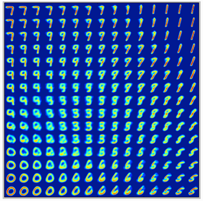
Generating digits using VAE.
Variational Autoencoder (VAE) vs. Generative Adversarial Networks (GAN)
Both VAE and GANs are very exciting approaches to learning the underlying data distribution using unsupervised learning GANs yield better results as compared to VAE.

Network architecture of VAE and GAN.
A GAN’s generator samples from a relatively low dimensional random variable and produces an image. Then the discriminator takes that image and predicts whether the image belongs to a target distribution or not. Once trained, I can generate a variety of images just by sampling the initial random variable and forwarding it through the generator.
A VAE’s encoder takes an image from a target distribution and compresses it into a low-dimensional latent space. Then the decoder’s job is to take that latent space representation and reproduce the original image. Once the network is trained, I can generate latent space representations of various images and interpolate between these before forwarding them through the decoder, which produces new images.
They are different techniques as they optimize different objective functions. It’s not like one of them will win across all of these situations. They will be useful in different situations. The objective function a learning method optimizes should ideally match the task we want to apply them for. In this sense, theory suggests that:
- GANs should be best at generating nice-looking samples — avoiding generating samples that don’t look plausible, at the cost of potentially underestimating the entropy of data.
- VAEs should be best at compressing data, as they maximize (a lower bound to) the likelihood. That said, evaluating the likelihood in VAE models is intractable, so it cannot be used very directly for direct entropy encoding.
- There are many models these days where the likelihood can be computed, such as pixel-RNNs, spatial LSTMs, RIDE, NADE, NICE, etc. These should also be best in terms of compression performance (shortest average codelength under lossless entropy coding).
I would recommend one paper comparing GANs and VAEs models: A Probe Towards Understanding GAN and VAE Models
Conclusion
As we have seen in this article, an autoencoder is a neural network architecture capable of pioneering structure within data in order to develop a compressed representation of the input data/image. Many different variants of the general autoencoder architecture exist with the goal of ensuring that the compressed representation represents significant traits of the original input data; typically, the biggest defiance when working with autoencoder is getting your model to actually learn a meaningful and generalizable latent space representation.
We also looked at how variational autoencoders perform better at generalizing a meaningful representation and can also be used as a generative model. Further, we saw how VAEs are different from generative adversarial networks (GANs).
Credits:
- https://www.jeremyjordan.me/variational-autoencoders/
- https://www.countbayesie.com/blog/2017/5/9/kullback-leibler-divergence-explained
- https://blog.keras.io/building-autoencoders-in-keras.html
- https://towardsdatascience.com/understanding-variational-autoencoders-vaes-f70510919f73
Original. Reposted with permission.
Related: