Photo by Marques Thomas on Unsplash

Introduction

The project’s goal is to partially recreate the Amazon Product Recommender System for the Electronics product category.

It’s November and Black Friday is here! What type of shopper are you? Do you save all the products you would like to buy for the day or would you rather open the website and see the live offers with their great discounts?

Even though online shops have been incredibly successful in the past decade, showing huge potential and growth, one of the fundamental differences between a physical and online store is the consumers’ impulse purchases.

If clients are presented with an assortment of products, they’re much more likely to purchase an item they didn’t originally plan on purchasing. The phenomenon of impulse buying is incredibly limited by the configuration of an online store. The same does not happen for their physical counterparts. The biggest physical retail chains make their customers go through a precise path to ensure they visit every aisle before exiting the store.

A way online stores like Amazon thought could recreate an impulse buying phenomenon is through recommender systems. Recommender systems identify the most similar or complementary products the customer just bought or viewed. The intent is to maximize the random purchases phenomenon that online stores normally lack.

Purchasing on Amazon made me quite interested in the mechanics and I wanted to re-create (even partially) the results of their recommender system.

According to the blog “Recostream”, the Amazon product recommender system has three types of dependencies, one of them being product-to-product recommendations. When a user has virtually no search history, the algorithm clusters products together and suggests them to that same user based on the items’ metadata.

The Data

The first step of the project is gathering the data. Luckily, the researchers at the University of California in San Diego have a repository to let the students, and individuals outside of the organization, use the data for research and projects. Data can be accessed through the following link along with many other interesting datasets related to recommender systems[2][3]. The product metadata was last updated in 2014; a lot of the products might not be available today.

The electronics category metadata contains 498,196 records and has 8 columns in total:

• asin — the unique ID associated with each product
• imUrl — the URL link of the image associated with each product
• description — The product’s description
• categories — a python list of all the categories each product falls into
• title — the title of the product
• price — the price of the product
• salesRank — the ranking of each product within a specific category
• related — products viewed and bought by customers related to each product
• brand — the brand of the product.

You will notice that the file is in a “loose” JSON format, where each line is a JSON containing all the columns previously mentioned as one of the fields. We’ll see how to deal with this in the code deployment section.

EDA

Let’s start with a quick Exploratory Data Analysis. After cleaning all the records that contained at least a NaN value in one of the columns, I created the visualizations for the electronics category.

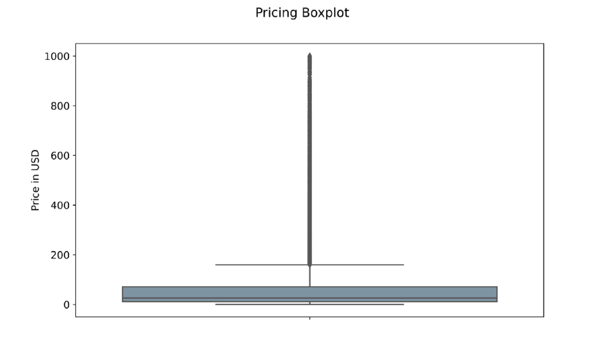
Price Boxplot with Outliers — Image by Author

The first chart is a boxplot showing the maximum, minimum, 25th percentile, 75th percentile, and average price of each product. For example, we know the maximum worth of a product is going to be $1000, whereas the minimum is around $1. The line above the $160 mark is made of dots, and each of these dots identifies an outlier. An outlier represents a record only happening once in the whole dataset. As a result, we know that there is only 1 product priced at around $1000.

The average price seems to be around the $25 mark. It is important to note that the library matplotlib automatically excludes outliers with the optionshowfliers=False. In order to make our boxplot look cleaner we can set the parameter equal to false.

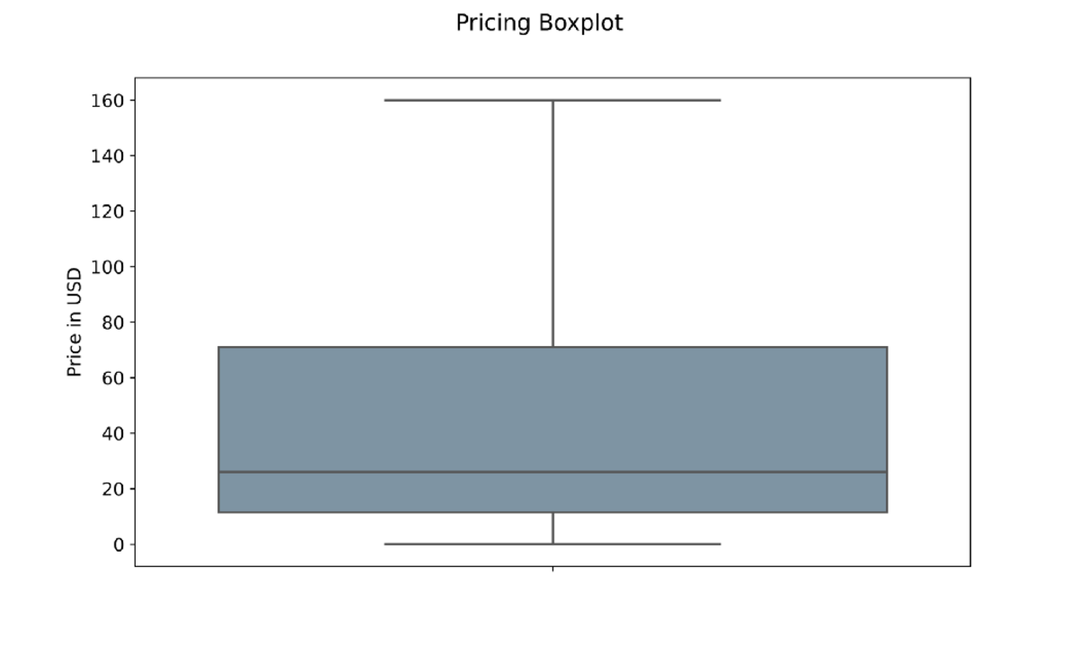
Price Boxplot — Image by Author

The result is a much cleaner Boxplot without the outliers. The chart also suggests that the vast majority of electronics products are priced around the $1 to $160 range.

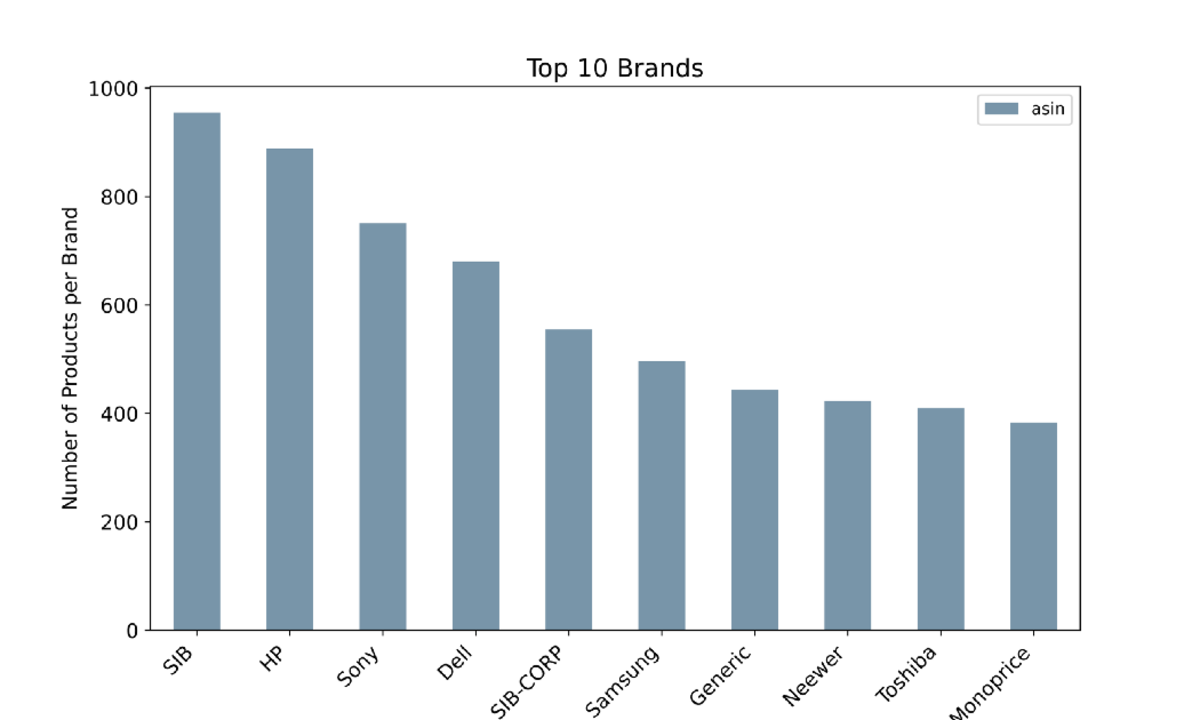
Top 10 Brands by Number of Products Listed — Image by Author

The chart shows the top 10 brands by the number of listed products selling on Amazon within the Electronics category. Among them, there are HP, Sony, Dell, and Samsung.

Top 10 Retailers Pricing Boxplot — Image by Author

Finally, we can see the price distribution for each of the top 10 sellers. Sony and Samsung definitely offer a wide range of products, from a few dollars all the way to $500 and $600, as a result, their average price is higher than most of the top competitors. Interestingly enough, SIB and SIB-CORP offer more products but at a much more affordable price on average.

The chart also tells us that Sony offers products that are roughly 60% of the highest-priced product in the dataset.

Cosine Similarity

A possible solution to cluster products together by their characteristics is cosine similarity. We need to understand this concept thoroughly to then build our recommender system.

Cosine similarity measures how “close” two sequences of numbers are. How does it apply to our case? Amazingly enough, sentences can be transformed into numbers, or better, into vectors.

Cosine similarity can take values between -1 and 1, where 1 indicates two vectors are formally the same whereas -1 indicates they’re as different as they can get.

Mathematically, cosine similarity is the dot product of two multidimensional vectors divided by the product of their magnitude [4]. I understand there are a lot of bad words in here but let’s try to break it down using a practical example.

Let’s suppose we’re analyzing document A and document B. Document A has three most common terms: “today”, “good”, and “sunshine” which respectively appear 4, 2, and 3 times. The same three terms in document B appear 3, 2, and 2 times. We can therefore write them like the following:

A = (2, 2, 3) ; B = (3, 2, 2)

The formula for the dot product of two vectors can be written as:

Their vector dot product is no other than 2x3 + 2x2 + 3x2 = 16

The single vector magnitude on the other hand is calculated as:

If I apply the formula I get

||A|| = 4.12 ; ||B|| = 4.12

their cosine similarity is therefore

16 / 17 = 0.94 = 19.74°

the two vectors are very similar.

As of now, we calculated the score only between two vectors with three dimensions. A word vector can virtually have an infinite number of dimensions (depending on how many words it contains) but the logic behind the process is mathematically the same. In the next section, we’ll see how to apply all the concepts in practice.

Code Deployment

Let’s move on to the code deployment phase to build our recommender system on the dataset.

Importing the libraries

The first cell of every data science notebook should import the libraries, the ones we need for the project are:

#Importing libraries for data management

import gzip
import json
import pandas as pd
from tqdm import tqdm_notebook as tqdm

#Importing libraries for feature engineering
import nltk
import re
from nltk.corpus import stopwords
from sklearn.feature_extraction.text import CountVectorizer 
from sklearn.metrics.pairwise import cosine_similarity

• gzip unzips the data files
• json decodes them
• pandas transforms JSON data into a more manageable dataframe format
• tqdm creates progress bars
• nltk to process text strings
• re provides regular expression support
• finally, sklearn is needed for text pre-processing

Reading the data

As previously mentioned, the data has been uploaded in a loose JSON format. The solution to this issue is first to transform the file into JSON readable format lines with the command json.dumps . Then, we can transform this file into a python list made of JSON lines by setting \n as the linebreak. Finally, we can append each line to the data empty list while reading it as a JSON with the command json.loads .

With the command pd.DataFrame the data list is read as a dataframe that we can now use to build our recommender.

#Creating an empty list
data = []

#Decoding the gzip file
def parse(path):
  g = gzip.open(path, 'r')
  for l in g:
    yield json.dumps(eval(l))

#Defining f as the file that will contain json data
f = open("output_strict.json", 'w')

#Defining linebreak as '\n' and writing one at the end of each line
for l in parse("meta_Electronics.json.gz"):
  f.write(l + '\n')

#Appending each json element to the empty 'data' list
with open('output_strict.json', 'r') as f:
    for l in tqdm(f):
        data.append(json.loads(l))

#Reading 'data' as a pandas dataframe
full = pd.DataFrame(data)

To give you an idea of how each line of the data list looks like we can run a simple command print(data[0]) , the console prints the line at index 0.

print(data[0])

output: 
{
'asin': '0132793040', 
'imUrl': 'http://ecx.images-amazon.com/images/I/31JIPhp%2BGIL.jpg', 
'description': 'The Kelby Training DVD Mastering Blend Modes in Adobe Photoshop CS5 with Corey Barker is a useful tool for...and confidence you need.', 
'categories': [['Electronics', 'Computers & Accessories', 'Cables & Accessories', 'Monitor Accessories']], 
'title': 'Kelby Training DVD: Mastering Blend Modes in Adobe Photoshop CS5 By Corey Barker'
}

As you can see the output is a JSON file, it has the {} to open and close the string, and each column name is followed by the : and the correspondent string. You can notice this first product is missing the price, salesRank, related, and brand information . Those columns are automatically filled with NaN values.

Once we read the entire list as a dataframe, the electronics products show the following 8 features:

| asin   | imUrl   | description   | categories   |
|--------|---------|---------------|--------------|
| price   | salesRank   | related   | brand   |
|---------|-------------|-----------|---------|

Feature Engineering

Feature engineering is responsible for data cleaning and creating the column in which we’ll calculate the cosine similarity score. Because of RAM memory limitations, I didn’t want the columns to be particularly long, as a review or product description could be. Conversely, I decided to create a “data soup” with the categories, title, and brand columns. Before that though, we need to eliminate every single row that contains a NaN value in either one of those three columns.

The selected columns contain valuable and essential information in the form of text we need for our recommender. The description column could also be a potential candidate but the string is often too long and it’s not standardized across the entire dataset. It doesn’t represent a reliable enough piece of information for what we’re trying to accomplish.

#Dropping each row containing a NaN value within selected columns
df = full.dropna(subset=['categories', 'title', 'brand'])

#Resetting index count
df = df.reset_index()

After running this first portion of code, the rows vertiginously decrease from 498,196 to roughly 142,000, a big change. It’s only at this point we can create the so-called data soup:

#Creating datasoup made of selected columns
df['ensemble'] = df['title'] + ' ' + 
df['categories'].astype(str) + ' ' + 
df['brand']

#Printing record at index 0
df['ensemble'].iloc[0]

output: 
"Barnes & Noble NOOK Power Kit in Carbon BNADPN31 
[['Electronics', 'eBook Readers & Accessories', 'Power Adapters']] 
Barnes & Noble"

The name of the brand needs to be included since the title does not always contain it.

Now I can move on to the cleaning portion. The function text_cleaning is responsible for removing every amp string from the ensemble column. On top of that, the string[^A-Za-z0–9] filters out every special character. Finally, the last line of the function eliminates every stopword the string contains.

#Defining text cleaning function
def text_cleaning(text):
    forbidden_words = set(stopwords.words('english'))
    text = re.sub(r'amp','',text)
    text = re.sub(r'\s+', ' ', re.sub('[^A-Za-z0-9]', ' ', 
           text.strip().lower())).strip()
    text = [word for word in text.split() if word not in forbidden_words]
    return ' '.join(text)

With the lambda function, we can apply text_cleaning to the entire column called ensemble , we can randomly select a data soup of a random product by calling iloc and indicating the index of the random record.

#Applying text cleaning function to each row
df['ensemble'] = df['ensemble'].apply(lambda text: text_cleaning(text))

#Printing line at Index 10000
df['ensemble'].iloc[10000]

output:
'vcool vga cooler electronics computers accessories 
computer components fans cooling case fans antec'

The record on the 10001st row (indexing starts from 0) is the vcool VGA cooler from Antec. This is a scenario in which the brand name was not in the title.

Cosine Computation and Recommender Function

The computation of cosine similarity starts with building a matrix containing all the words that ever appear in the ensemble column. The method we’re going to use is called “Count Vectorization” or more commonly “Bag of words”. If you’d like to read more about count vectorization, you can read one of my previous articles at the following link.

Because of RAM limitations, the cosine similarity score will be computed only on the first 35,000 records out of the 142,000 available after the pre-processing phase. This most likely affects the final performance of the recommender.

#Selecting first 35000 rows
df = df.head(35000)

#creating count_vect object
count_vect = CountVectorizer()

#Create Matrix
count_matrix = count_vect.fit_transform(df['ensemble'])

# Compute the cosine similarity matrix
cosine_sim = cosine_similarity(count_matrix, count_matrix)

The command cosine_similarity , as the name suggests, calculates cosine similarity for each line in the count_matrix . Each line on the count_matrix is no other than a vector with the word count of every word that appears in the ensemble column.

#Creating a Pandas Series from df's index
indices = pd.Series(df.index, index=df['title']).drop_duplicates()

Before running the actual recommender system, we need to make sure to create an index and that this index has no duplicates.

It’s only at this point we can define the content_recommenderfunction. It has 4 arguments: title, cosine_sim, df, and indices. The title will be the only element to input when calling the function.

content_recommender works in the following way:

• It finds the product’s index associated with the title the user provides
• It searches the product’s index within the cosine similarity matrix and gathers all the scores of all the products
• It sorts all the scores from the most similar product (closer to 1) to the least similar (closer to 0)
• It only selects the first 30 most similar products
• It adds an index and returns a pandas series with the result

# Function that takes in product title as input and gives recommendations
def content_recommender(title, cosine_sim=cosine_sim, df=df,
indices=indices):
        
    # Obtain the index of the product that matches the title
    idx = indices[title]
        
    # Get the pairwsie similarity scores of all products with that product
    # And convert it into a list of tuples as described above
    sim_scores = list(enumerate(cosine_sim[idx]))
        
    # Sort the products based on the cosine similarity scores
    sim_scores = sorted(sim_scores, key=lambda x: x[1], reverse=True)
        
    # Get the scores of the 30 most similar products. Ignore the first product.
    sim_scores = sim_scores[1:30]
        
    # Get the product indices
    product_indices = [i[0] for i in sim_scores]
        
    # Return the top 30 most similar products
    return df['title'].iloc[product_indices]

Now let’s test it on the “Vcool VGA Cooler”. We want 30 products that are similar and customers would be interested in buying. By running the command content_recommender(product_title) , the function returns a list of 30 recommendations.

#Define the product we want to recommend other items from
product_title = 'Vcool VGA Cooler'

#Launching the content_recommender function
recommendations = content_recommender(product_title)

#Associating titles to recommendations
asin_recommendations = df[df['title'].isin(recommendations)]

#Merging datasets
recommendations = pd.merge(recommendations, 
                           asin_recommendations, 
                           on='title', 
                           how='left')

#Showing top 5 recommended products
recommendations['title'].head()

Among the 5 most similar products we find other Antec products such as the Tricool Computer Case Fan, the Expansion Slot Cooling Fan, and so forth.

1    Antec Big Boy 200 - 200mm Tricool Computer Case Fan                                                            
2    Antec Cyclone Blower, Expansion Slot Cooling Fan                                                               
3    StarTech.com 90x25mm High Air Flow Dual Ball Bearing Computer Case Fan with TX3 Cooling Fan FAN9X25TX3H (Black)
4    Antec 120MM BLUE LED FAN Case Fan (Clear)                                                                      
5    Antec PRO 80MM 80mm Case Fan Pro with 3-Pin & 4-Pin Connector (Discontinued by Manufacturer)

The related column in the original dataset contains a list of products consumers also bought, bought together, and bought after viewing the VGA Cooler.

#Selecting the 'related' column of the product we computed recommendations for
related = pd.DataFrame.from_dict(df['related'].iloc[10000], orient='index').transpose()

#Printing first 10 records of the dataset
related.head(10)

By printing the head of the python dictionary in that column the console returns the following dataset.

|    | also_bought   | bought_together   | buy_after_viewing   |
|---:|:--------------|:------------------|:--------------------|
|  0 | B000051299    | B000233ZMU        | B000051299          |
|  1 | B000233ZMU    | B000051299        | B00552Q7SC          |
|  2 | B000I5KSNQ    |                   | B000233ZMU          |
|  3 | B00552Q7SC    |                   | B004X90SE2          |
|  4 | B000HVHCKS    |                   |                     |
|  5 | B0026ZPFCK    |                   |                     |
|  6 | B009SJR3GS    |                   |                     |
|  7 | B004X90SE2    |                   |                     |
|  8 | B001NPEBEC    |                   |                     |
|  9 | B002DUKPN2    |                   |                     |
| 10 | B00066FH1U    |                   |                     |

Let’s test if our recommender did well. Let’s see if some of the asin ids in the also_bought list are present in the recommendations.

#Checking if recommended products are in the 'also_bought' column for
#final evaluation of the recommender

related['also_bought'].isin(recommendations['asin'])

Our recommender correctly suggested 5 out of 44 products.

[True False  True False False False False False False False  True False False False False False False  True False False False False False False False False  True False False False False False False False False False False False False False False False False False]

I agree it’s not an optimal result but considering we only used 35,000 out of the 498,196 rows available in the full dataset, it’s acceptable. It certainly has a lot of room for improvement. If NaN values were less frequent or even non-existent for target columns, recommendations could be more accurate and close to the actual Amazon ones. Secondly, having access to larger RAM memory, or even distributed computing, could allow the practitioner to compute even larger matrices.

Conclusion

I hope you enjoyed the project and that it’ll be useful for any future use.

As mentioned in the article, the final result can be further improved by including all lines of the dataset in the cosine similarity matrix. On top of that, we could add each product’s review average score by merging the metadata dataset with others available in the repository. We could include the price in the computation of the cosine similarity. Another possible improvement could be building a recommender system completely based on each product’s descriptive images.

The main solutions for further improvements have been listed. Most of them are even worth pursuing from the perspective of future implementation into actual production.

As a final note, if you liked the content please consider dropping a follow to be notified when new articles are published. If you have any observations about the article, write them in the comments! I’d love to read them :) Thank you for reading!

PS: If you like my writing, it would mean the world to me if you could subscribe to a medium membership through this link. With the membership, you get the amazing value that medium articles provide and it’s an indirect way of supporting my content!

Reference

[1] Amazon’s Product Recommendation System In 2021: How Does The Algorithm Of The eCommerce Giant Work? — Recostream. (2021). Retrieved November 1, 2022, from Recostream.com website: https://recostream.com/blog/amazon-recommendation-system

[2] He, R., & McAuley, J. (2016, April). Ups and downs: Modeling the visual evolution of fashion trends with one-class collaborative filtering. In Proceedings of the 25th international conference on world wide web (pp. 507–517).

[3] McAuley, J., Targett, C., Shi, Q., & Van Den Hengel, A. (2015, August). Image-based recommendations on styles and substitutes. In Proceedings of the 38th international ACM SIGIR conference on research and development in information retrieval (pp. 43–52).

[4] Rahutomo, F., Kitasuka, T., & Aritsugi, M. (2012, October). Semantic cosine similarity. In The 7th international student conference on advanced science and technology ICAST (Vol. 4, ?1, p. 1).

[5] Rounak Banik. 2018. Hands-On Recommendation Systems with Python: Start building powerful and personalized, recommendation engines with Python. Packt Publishing.

 
 
Giovanni Valdata holds two BBAs and a Msc. in Management, at the end of which leveraged NLP for his thesis in Data Science and Management. Giovanni enjoys helping readers to learn more about the field by developing technical projects with practical applications.

 
Original. Reposted with permission.