 Complete Guide to Build ConvNet HTTP-Based Application using TensorFlow and Flask RESTful Python API
 Complete Guide to Build ConvNet HTTP-Based Application using TensorFlow and Flask RESTful Python API
In this tutorial, a CNN is to be built, and trained and tested against the CIFAR10 dataset. To make the model remotely accessible, a Flask Web application is created using Python to receive an uploaded image and return its classification label using HTTP.
This tutorial takes you along the steps required to create a convolutional neural network (CNN/ConvNet) using TensorFlow and get it into production by allowing remote access via a HTTP-based application using Flask RESTful API.
In this tutorial, a CNN is to be built using TensorFlow NN (tf.nn) module. The CNN model architecture is created and trained and tested against the CIFAR10 dataset. To make the model remotely accessible, a Flask Web application is created using Python to receive an uploaded image and return its classification label using HTTP. Anaconda3 is used in addition to TensorFlow on Windows with CPU support. This tutorial assumes you have a basic understanding of CNN such as layers, strides, and padding. Also knowledge about Python is required.
The tutorial is summarized into the following steps:
- Preparing the Environment by Installing Python, TensorFlow, PyCharm, and Flask API.
- Downloading and Preparing the CIFAR-10 Dataset.
- Building the CNN Computational Graph using TensorFlow.
- Training the CNN.
- Saving the Trained CNN Model.
- Preparing the Test Data and Restoring the Trained CNN Model.
- Testing the Trained CNN Model.
- Building the Flask Web Application.
- Upload an Image using HTML Form.
- Creating Helper HTML, JavaScript, and CSS Files.
- HTTP-Based Remote Accessing the Trained Model for Prediction.
1. Installing Python, TensorFlow, PyCharm, and Flask API
Before starting building the project, it is required to prepare its environment. Python is the first tool to start installing because the environment is fully dependent on it. If you already have the environment prepared, you can skip the first step.
1.1 Anaconda/Python Installation
It is possible to install the native Python distribution but it is recommended to use an all-in-one package such as Anaconda because it does some stuff for you. In this project, Anaconda 3 is used. For Windows, the executable file can be downloaded from https://www.anaconda.com/download/#windows. It could be installed easily.
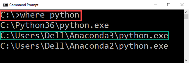
To ensure Anaconda3 is installed properly, the CMD command (where python) could be issued as in figure 1. If Anaconda3 is installed properly, its installation path will appear in the command output.
Figure 1
1.2 TensorFlow Installation
After installation Python using Anaconda3, next is to install TensorFlow (TF). This tutorial uses TF on Windows with CPU support. The installation instructions are found in this page https://www.tensorflow.org/install/install_windows. This YouTube video might be helpful (https://youtu.be/MsONo20MRVU).
TF installation steps are as follows:
1) Creating a conda environment for TF by invoking this command:
C:> conda create -n tensorflow pip python=3.5
This creates an empty folder holding the virtual environment (venv) for TF installation. The venv is located under Anaconda3 installation directory in this location (\Anaconda3\envs\tensorflow).
2) Activating the venv for TensorFlow installation using this command:
C:> activate tensorflow
The above command tells that we are inside the venv and any library installation will be inside it. The command prompt is expected to be changed after this command to be (tensorflow)C:>. After getting into the directory, we are ready to install the library.
3) After activating the venv, the CPU-only version of Windows TensorFlow could be installed by issuing this command:
(tensorflow)C:> pip install --ignore-installed --upgrade tensorflow
To test whether TF is installed properly, we can try to import it as in figure 2. But remember before importing TF, its venv must be activated. Testing it from the CMD, we need to issue the python command in order to be able to interact with Python. Because no error occurred in the import line, TF is successfully installed.
Figure 2

1.3 PyCharm Python IDE Installation
For this project, it is recommended to use a Python IDE rather than entering commands in CMD. The IDE used in this tutorial is PyCharm. Its Windows executable file could be downloaded from this page https://www.jetbrains.com/pycharm/download/#section=windows. Its installation instructions are pretty simple.
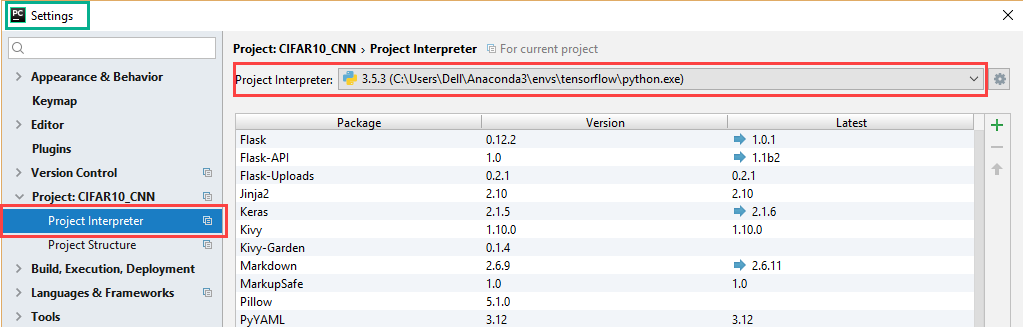
After downloading and installation PyCharm Python IDE, next is to link it with TF. This is done by setting its Python interpreter to the installed Python under the TF venv as in figure 3. This is done by opening the settings of the IDE and choosing the Project interpreter to the python.exe file installed inside the TF venv.
Figure 3
1.4 Flask Installation
The last tool to get installed is the Flask RESTful API. It is a library to be installed using pip/conda installer under the TF venv using the following CMD command:
C:> pip install Flask-API
If not already installed, NumPy and SciPy should be installed inside the venv in order to be able to read and manipulate images.
By installing Anaconda (Python), TensorFlow, PyCharm, and Flask, we are ready to start building the project.
2. Downloading and Preparing the CIFAR-10 Dataset
The Python version of the 10 classes CIFAR dataset (CIFAR-10) could be downloaded from this page https://www.cs.toronto.edu/~kriz/cifar.html. The dataset contains 60,000 images divided into training and testing data. There are five files holding the training data where each file has 10,000 images. The images are RGB of size 32x32x3. The training files are named data_batch_1, data_batch_2, and so on. There is a single file holding the test data named test_batch with 10,000 images. A metadata file named batches.meta is available that holds the dataset classes labels which are airplane, automobile, bird, cat, deer, dog, frog, horse, ship, and truck.
Because each file in the dataset is a binary file, it should be decoded in order to retrieve the actual image data. For such reason, a function called unpickle_patch is created to do such job defined as follows:
def unpickle_patch(file):

    """
    Decoding the binary file.
    :param file:File to decode it data.
    :return:Dictionary of the file holding details including input data and output labels.
    """
    patch_bin_file = open(file, 'rb')#Reading the binary file.
    patch_dict = pickle.load(patch_bin_file, encoding='bytes')#Loading the details of the binary file into a dictionary.
    return patch_dict#Returning the dictionary.
The method accepts the binary file name and returns a dictionary holding details about such file. The dictionary holds the data for all 10,000 samples within the file in addition to their labels.
In order to decode the entire training data, a new function called get_dataset_images is created. That function accepts the dataset path and works only on the training data. As a result, it filters the files under this path and returns only files starting with data_batch_. The testing data is prepared later after building and training the CNN.
For each training file, it is decoded by calling the unpickle_patch function. Based on the dictionary returned by such function, the get_dataset_images function returns both the images data and their class labels. The images data is retrieved from the ‘data’ key and their class labels are retrieved from the ‘labels’ key.
Because the images data are saved as 1D vector, it should be reshaped to be of 3 dimensions. This is because TensorFlow accepts the images of such shape. For such reason, the get_dataset_images function accepts the number of rows/columns in addition to the number of channels in each image as arguments.
The implementation of such function is as follows:
def get_dataset_images(dataset_path, im_dim=32, num_channels=3):

    """
    This function accepts the dataset path, reads the data, and returns it after being reshaped to match the requierments of the CNN.
    :param dataset_path:Path of the CIFAR10 dataset binary files.
    :param im_dim:Number of rows and columns in each image. The image is expected to be rectangular.
    :param num_channels:Number of color channels in the image.
    :return:Returns the input data after being reshaped and output labels.
    """
    num_files = 5#Number of training binary files in the CIFAR10 dataset.
    images_per_file = 10000#Number of samples withing each binary file.
    files_names = os.listdir(patches_dir)#Listing the binary files in the dataset path.
    """
    Creating an empty array to hold the entire training data after being reshaped.
    The dataset has 5 binary files holding the data. Each binary file has 10,000 samples. Total number of samples in the dataset is 5*10,000=50,000.
    Each sample has a total of 3,072 pixels. These pixels are reshaped to form a RGB image of shape 32x32x3.
    Finally, the entire dataset has 50,000 samples and each sample of shape 32x32x3 (50,000x32x32x3).
    """
    dataset_array = numpy.zeros(shape=(num_files * images_per_file, im_dim, im_dim, num_channels))
    #Creating an empty array to hold the labels of each input sample. Its size is 50,000 to hold the label of each sample in the dataset.
    dataset_labels = numpy.zeros(shape=(num_files * images_per_file), dtype=numpy.uint8)
    index = 0#Index variable to count number of training binary files being processed.
    for file_name in files_names:
        """
        Because the CIFAR10 directory does not only contain the desired training files and has some  other files, it is required to filter the required files.
        Training files start by 'data_batch_' which is used to test whether the file is for training or not.
        """
        if file_name[0:len(file_name) - 1] == "data_batch_":
            print("Working on : ", file_name)
            """
            Appending the path of the binary files to the name of the current file.
            Then the complete path of the binary file is used to decoded the file and return the actual pixels values.
            """
            data_dict = unpickle_patch(dataset_path+file_name)
            """
            Returning the data using its key 'data' in the dictionary.
            Character b is used before the key to tell it is binary string.
            """
            images_data = data_dict[b"data"]
            #Reshaping all samples in the current binary file to be of 32x32x3 shape.
            images_data_reshaped = numpy.reshape(images_data, newshape=(len(images_data), im_dim, im_dim, num_channels))
            #Appending the data of the current file after being reshaped.
            dataset_array[index * images_per_file:(index + 1) * images_per_file, :, :, :] = images_data_reshaped
            #Appening the labels of the current file.
            dataset_labels[index * images_per_file:(index + 1) * images_per_file] = data_dict[b"labels"]
            index = index + 1#Incrementing the counter of the processed training files by 1 to accept new file.
    return dataset_array, dataset_labels#Returning the training input data and output labels.
By preparing the training data, we can build and train the CNN model using TF.
3. Building the CNN Computational Graph using TensorFlow
The computational graph of the CNN is created inside a function called create_CNN. It creates a stack of convolution (conv), ReLU, max pooling, dropout, and fully connected (FC) layers and returns the results of the last fully connected layer. The output of each layer is the input to the next layer. This requires consistency between the sizes of outputs and inputs of neighboring layers. Note that for each conv, ReLU, and max pooling layers, there are some of parameters to get specified such as strides across each dimension and padding.
def create_CNN(input_data, num_classes, keep_prop):

    """
    Builds the CNN architecture by stacking conv, relu, pool, dropout, and fully connected layers.
    :param input_data:patch data to be processed.
    :param num_classes:Number of classes in the dataset. It helps determining the number of outputs in the last fully connected layer.
    :param keep_prop:probability of dropping neurons in the dropout layer.
    :return: last fully connected layer.
    """
    #Preparing the first convolution layer.
    filters1, conv_layer1 = create_conv_layer(input_data=input_data, filter_size=5, num_filters=4)
    """
    Applying ReLU activation function over the conv layer output.
    It returns a new array of the same shape as the input array.
    """
    relu_layer1 = tensorflow.nn.relu(conv_layer1)
    print("Size of relu1 result : ", relu_layer1.shape)
    """
    Max pooling is applied to the ReLU layer result to achieve translation invariance.
    It returns a new array of a different shape from the the input array relative to the strides and kernel size used.
    """
    max_pooling_layer1 = tensorflow.nn.max_pool(value=relu_layer1,
                                                ksize=[1, 2, 2, 1],
                                                strides=[1, 1, 1, 1],
                                                padding="VALID")
    print("Size of maxpool1 result : ", max_pooling_layer1.shape)

    #Similar to the previous conv-relu-pool layers, new layers are just stacked to complete the CNN architecture.
    #Conv layer with 3 filters and each filter is of sisze of 5x5.
    filters2, conv_layer2 = create_conv_layer(input_data=max_pooling_layer1, filter_size=7, num_filters=3)
    relu_layer2 = tensorflow.nn.relu(conv_layer2)
    print("Size of relu2 result : ", relu_layer2.shape)
    max_pooling_layer2 = tensorflow.nn.max_pool(value=relu_layer2,
                                                ksize=[1, 2, 2, 1],
                                                strides=[1, 1, 1, 1],
                                                padding="VALID")
    print("Size of maxpool2 result : ", max_pooling_layer2.shape)

    #Conv layer with 2 filters and a filter sisze of 5x5.
    filters3, conv_layer3 = create_conv_layer(input_data=max_pooling_layer2, filter_size=5, num_filters=2)
    relu_layer3 = tensorflow.nn.relu(conv_layer3)
    print("Size of relu3 result : ", relu_layer3.shape)
    max_pooling_layer3 = tensorflow.nn.max_pool(value=relu_layer3,
                                                ksize=[1, 2, 2, 1],
                                                strides=[1, 1, 1, 1],
                                                padding="VALID")
    print("Size of maxpool3 result : ", max_pooling_layer3.shape)

    #Adding dropout layer before the fully connected layers to avoid overfitting.
    flattened_layer = dropout_flatten_layer(previous_layer=max_pooling_layer3, keep_prop=keep_prop)

    #First fully connected (FC) layer. It accepts the result of the dropout layer after being flattened (1D).
    fc_resultl = fc_layer(flattened_layer=flattened_layer, num_inputs=flattened_layer.get_shape()[1:].num_elements(),
                          num_outputs=200)
    #Second fully connected layer accepting the output of the previous fully connected layer. Number of outputs is equal to the number of dataset classes.
    fc_result2 = fc_layer(flattened_layer=fc_resultl, num_inputs=fc_resultl.get_shape()[1:].num_elements(),
                          num_outputs=num_classes)
    print("Fully connected layer results : ", fc_result2)
    return fc_result2#Returning the result of the last FC layer.
Because the convolution layer applies the convolution operation between the input data and the set of filters used, the create_CNN function accepts the input data as an input argument. Such data is what returned by the get_dataset_images function. The convolution layer is created using the create_conv_layer function. The create_conv_layer function accepts the input data, filter size, and number of filters and returns the result of convolving the input data with the set of filters. The set of filters have their size set according to the depth of the input images. The create_conv_layer is defined as follows:
def create_conv_layer(input_data, filter_size, num_filters):

    """
    Builds the CNN convolution (conv) layer.
    :param input_data:patch data to be processed.
    :param filter_size:#Number of rows and columns of each filter. It is expected to have a rectangular filter.
    :param num_filters:Number of filters.
    :return:The last fully connected layer of the network.
    """
    """
    Preparing the filters of the conv layer by specifiying its shape.
    Number of channels in both input image and each filter must match.
    Because number of channels is specified in the shape of the input image as the last value, index of -1 works fine.
    """
    filters = tensorflow.Variable(tensorflow.truncated_normal(shape=(filter_size, filter_size, tensorflow.cast(input_data.shape[-1], dtype=tensorflow.int32), num_filters),
                                                              stddev=0.05))
    print("Size of conv filters bank : ", filters.shape)

    """
    Building the convolution layer by specifying the input data, filters, strides along each of the 4 dimensions, and the padding.
    Padding value of 'VALID' means the some borders of the input image will be lost in the result based on the filter size.
    """
    conv_layer = tensorflow.nn.conv2d(input=input_data,
                                      filter=filters,
                                      strides=[1, 1, 1, 1],
                                      padding="VALID")
    print("Size of conv result : ", conv_layer.shape)
    return filters, conv_layer#Returing the filters and the convolution layer result.
Another argument is the probability of keeping neurons in the dropout layer. It specifies how much neurons are dropped by the dropout layer. The dropout layer is implemented using the dropout_flatten_layer function as shown below. Such function returns a flattened array that will be the input to the fully connected layer.
def dropout_flatten_layer(previous_layer, keep_prop):

    """
    Applying the dropout layer.
    :param previous_layer: Result of the previous layer to the dropout layer.
    :param keep_prop: Probability of keeping neurons.
    :return: flattened array.
    """
    dropout = tensorflow.nn.dropout(x=previous_layer, keep_prob=keep_prop)
    num_features = dropout.get_shape()[1:].num_elements()
    layer = tensorflow.reshape(previous_layer, shape=(-1, num_features))#Flattening the results.
    return layer
Because the last FC layer should have number of output neurons equal to the number of dataset classes, the number of dataset classes is used as another input argument to the create_CNN function. The fully connected layer is created using the fc_layer function. Such function accepts the flattened result of the dropout layer, the number of features in such flattened result, and number of output neurons from such FC layer. Based on number of inputs and outputs, a weights tensor is created which get then multiplied by the flattened layer to get the returned result of the FC layer.
def fc_layer(flattened_layer, num_inputs, num_outputs):

    """
    uilds a fully connected (FC) layer.
    :param flattened_layer: Previous layer after being flattened.
    :param num_inputs: Number of inputs in the previous layer.
    :param num_outputs: Number of outputs to be returned in such FC layer.
    :return:
    """
    #Preparing the set of weights for the FC layer. It depends on the number of inputs and number of outputs.
    fc_weights = tensorflow.Variable(tensorflow.truncated_normal(shape=(num_inputs, num_outputs),
                                                              stddev=0.05))
    #Matrix multiplication between the flattened array and the set of weights.
    fc_resultl = tensorflow.matmul(flattened_layer, fc_weights)
    return fc_resultl#Output of the FC layer (result of matrix multiplication).
The computational graph after being visualized using TensorBoard is shown in figure 4.
Figure 4
