Deep Quantile Regression

comments

By Sachin Abeywardana, Founder of DeepSchool.io

One area that Deep Learning has not explored extensively is the uncertainty in estimates. Most Deep Learning frameworks currently focus on giving a best estimate as defined by a loss function. Occasionally something beyond a point estimate is required to make a decision. This is where a distribution would be useful. Bayesian statistics lends itself to this problem really well since a distribution over the dataset is inferred. However, Bayesian methods so far have been rather slow and would be expensive to apply to large datasets.

As far as decision making goes, most people actually require quantiles as opposed to true uncertainty in an estimate. For instance when measuring a child’s weight for a given age, the weight of an individual will vary. What would be interesting is (for arguments sake) the 10th and 90th percentile. Note that the uncertainty is different to quantiles in that I could request for a confidence interval on the 90th quantile. This article will purely focus on inferring quantiles.

Quantile Regression Loss function

 
In regression the most commonly used loss function is the mean squared error function. If we were to take the negative of this loss and exponentiate it, the result would correspond to the gaussian distribution. The mode of this distribution (the peak) corresponds to the mean parameter. Hence, when we predict using a neural net that minimised this loss we are predicting the mean value of the output which may have been noisy in the training set.

The loss in Quantile Regression for an individual data point is defined as:

Loss of individual data point

where alpha is the required quantile (a value between 0 and 1) and

where f(x) is the predicted (quantile) model and y is the observed value for the corresponding input x. The average loss over the entire dataset is shown below:

Loss funtion

If we were to take the negative of the individual loss and exponentiate it, we get the distribution know as the Asymmetric Laplace distribution, shown below. The reason that this loss function works is that if we were to find the area under the graph to the left of zero it would be alpha, the required quantile.

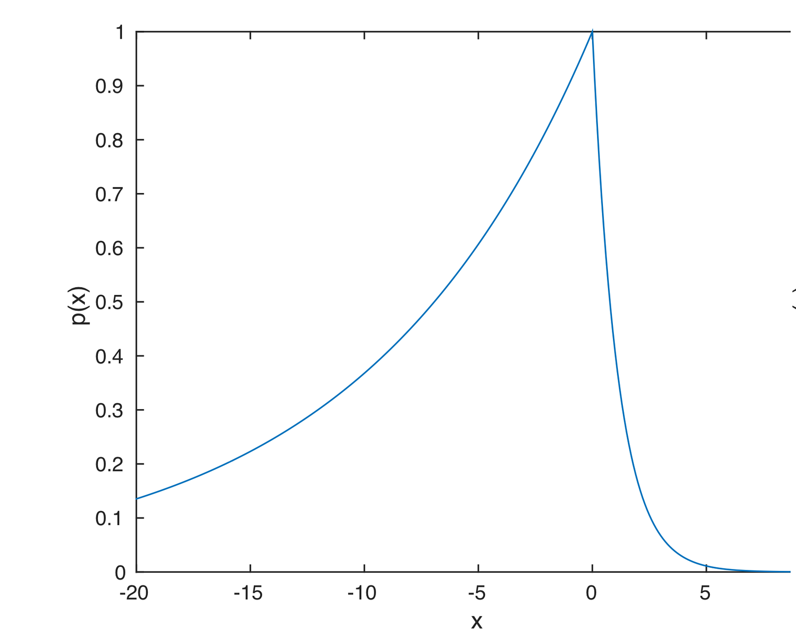
Probability distribution function (pdf) of an Asymmetric Laplace distribution.

The case when alpha=0.5 is most likely more familiar since it corresponds to the Mean Absolute Error (MAE). This loss function consistently estimates the median (50th percentile), instead of the mean.

Modelling in Keras

 
The forward model is no different to what you would have had when doing MSE regression. All that changes is the loss function. The following few lines defines the loss function defined in the section above.

import keras.backend as K
def tilted_loss(q,y,f):
    e = (y-f)
    return K.mean(K.maximum(q*e, (q-1)*e), axis=-1)

When it comes to compiling the neural network, just simply do:

quantile = 0.5
model.compile(loss=lambda y,f: tilted_loss(quantile,y,f), optimizer='adagrad')

For a full example see this Jupyter notebook where I look at a motor cycle crash dataset over time. The results are reproduced below where I show the 10th 50th and 90th quantiles.

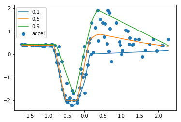
Acceleration over time of crashed motor cycle.

 
Final Notes

1. Note that for each quantile I had to rerun the training. This is due to the fact that for each quantile the loss function is different, as the quantile in itself is a parameter for the loss function.
2. Due to the fact that each model is a simple rerun, there is a risk of quantile cross over. i.e. the 49th quantile may go above the 50th quantile at some stage.
3. Note that the quantile 0.5 is the same as median, which you can attain by minimising Mean Absolute Error, which you can attain in Keras regardless with loss='mae'.
4. Uncertainty and quantiles are not the same thing. But most of the time you care about quantiles and not uncertainty.
5. If you really do want uncertainty with deep nets checkout http://mlg.eng.cam.ac.uk/yarin/blog_3d801aa532c1ce.html

 
Edit 1

As pointed out by Anders Christiansen (in the responses) we may be able to get multiple quantiles in one go by having multiple objectives. Keras however combines all loss functions by a loss_weights argument as shown here: https://keras.io/getting-started/functional-api-guide/#multi-input-and-multi-output-models. Would be easier to implement this in tensorflow. If anyone beats me to it would be happy to change my notebook/ post to reflect this. As a rough guide if we wanted the quantiles 0.1, 0.5, 0.9, the last layer in Keras would have Dense(3) instead, with each node connected to a loss function.

 
Edit 2

Thanks to Jacob Zweig for implementing the simultaneous multiple Quantiles in TensorFlow: https://github.com/strongio/quantile-regression-tensorflow/blob/master/Quantile%20Loss.ipynb

 
If you are enjoying my tutorials/ blog posts, consider supporting me on https://www.patreon.com/deepschoolio or by subscribing to my YouTube channel https://www.youtube.com/user/sachinabey (or both!).

 
Bio: Sachin Abeywardana is a PhD in Machine Learning and Founder of DeepSchool.io.

Original. Reposted with permission.

Related:

• DeepSchool.io: Deep Learning Learning
• Docker for Data Science
• Using Genetic Algorithm for Optimizing Recurrent Neural Networks