Machine Learning for Text Classification Using SpaCy in Python
In this post, we will demonstrate how text classification can be implemented using spaCy without having any deep learning experience.
By Susan Li, Sr. Data Scientist

Photo Credit: Pixabay
spaCy is a popular and easy-to-use natural language processing library in Python. It provides current state-of-the-art accuracy and speed levels, and has an active open source community. However, since SpaCy is a relative new NLP library, and it’s not as widely adopted as NLTK. There is not yet sufficient tutorials available.
In this post, we will demonstrate how text classification can be implemented using spaCy without having any deep learning experience.
The Data
It s often time consuming and frustrating experience for a young researcher to find and select a suitable academic conference to submit his (or her) academic papers. We define “suitable conference”, meaning the conference is aligned with the researcher’s work and have a good academic ranking.
Using the conference proceeding data set, we are going to categorize research papers by conferences. Let’s get started. The data set can be found here.
Explore
Take a quick peek:
import pandas as pd
import numpy as np
import seaborn as sns
import matplotlib.pyplot as plt
import base64
import string
import re
from collections import Counter
from nltk.corpus import stopwords
stopwords = stopwords.words('english')

df = pd.read_csv('research_paper.csv')
df.head()
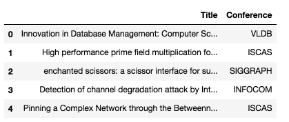
Figure 1
There is no missing values.
df.isnull().sum()
Title 0
Conference 0
dtype: int64
Split the data to train and test sets:
from sklearn.model_selection import train_test_split
train, test = train_test_split(df, test_size=0.33, random_state=42)

print('Research title sample:', train['Title'].iloc[0])
print('Conference of this paper:', train['Conference'].iloc[0])
print('Training Data Shape:', train.shape)
print('Testing Data Shape:', test.shape)
Research title sample: Cooperating with Smartness: Using Heterogeneous Smart Antennas in Ad-Hoc Networks.
Conference of this paper: INFOCOM
Training Data Shape: (1679, 2)
Testing Data Shape: (828, 2)
The dataset consists of 2507 short research paper titles, which have been classified into 5 categories (by conferences). The following figure summarizes the distribution of research papers by different conferences.
fig = plt.figure(figsize=(8,4))
sns.barplot(x = train['Conference'].unique(), y=train['Conference'].value_counts())
plt.show()
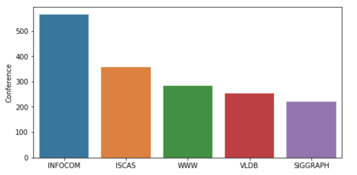
Figure 2
The following is one way to do text preprocessing in SpaCy. After that, we are trying to find out the top words used in the papers that submit to the first and second categories (conferences) — INFOCOM & ISCAS
import spacy

nlp = spacy.load('en_core_web_sm')
punctuations = string.punctuation

def cleanup_text(docs, logging=False):
    texts = []
    counter = 1
    for doc in docs:
        if counter % 1000 == 0 and logging:
            print("Processed %d out of %d documents." % (counter, len(docs)))
        counter += 1
        doc = nlp(doc, disable=['parser', 'ner'])
        tokens = [tok.lemma_.lower().strip() for tok in doc if tok.lemma_ != '-PRON-']
        tokens = [tok for tok in tokens if tok not in stopwords and tok not in punctuations]
        tokens = ' '.join(tokens)
        texts.append(tokens)
    return pd.Series(texts)

INFO_text = [text for text in train[train['Conference'] == 'INFOCOM']['Title']]

IS_text = [text for text in train[train['Conference'] == 'ISCAS']['Title']]

INFO_clean = cleanup_text(INFO_text)
INFO_clean = ' '.join(INFO_clean).split()

IS_clean = cleanup_text(IS_text)
IS_clean = ' '.join(IS_clean).split()

INFO_counts = Counter(INFO_clean)
IS_counts = Counter(IS_clean)

INFO_common_words = [word[0] for word in INFO_counts.most_common(20)]
INFO_common_counts = [word[1] for word in INFO_counts.most_common(20)]

fig = plt.figure(figsize=(18,6))
sns.barplot(x=INFO_common_words, y=INFO_common_counts)
plt.title('Most Common Words used in the research papers for conference INFOCOM')
plt.show()
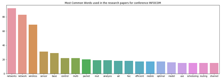
Figure 3
IS_common_words = [word[0] for word in IS_counts.most_common(20)]
IS_common_counts = [word[1] for word in IS_counts.most_common(20)]

fig = plt.figure(figsize=(18,6))
sns.barplot(x=IS_common_words, y=IS_common_counts)
plt.title('Most Common Words used in the research papers for conference ISCAS')
plt.show()
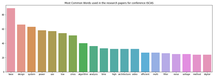
Figure 4
The top words in INFOCOM are “networks” and “network”. It is obvious that INFOCOM is a conference in the field of networking and closely related areas.
The top words in ISCAS are “base” and “design”. It indicates that ISCAS is a conference about database, system design and related topics.
Machine Learning with spaCy
from sklearn.feature_extraction.text import CountVectorizer
from sklearn.base import TransformerMixin
from sklearn.pipeline import Pipeline
from sklearn.svm import LinearSVC
from sklearn.feature_extraction.stop_words import ENGLISH_STOP_WORDS
from sklearn.metrics import accuracy_score
from nltk.corpus import stopwords
import string
import re
import spacy
spacy.load('en')
from spacy.lang.en import English
parser = English()
Below is another way to clean text using spaCy:
STOPLIST = set(stopwords.words('english') + list(ENGLISH_STOP_WORDS))
SYMBOLS = " ".join(string.punctuation).split(" ") + ["-", "...", "”", "”"]

class CleanTextTransformer(TransformerMixin):

   def transform(self, X, **transform_params):
        return [cleanText(text) for text in X]

   def fit(self, X, y=None, **fit_params):
        return self

   def get_params(self, deep=True):
        return {}

def cleanText(text):
    text = text.strip().replace("\n", " ").replace("\r", " ")
    text = text.lower()

def tokenizeText(sample):
    tokens = parser(sample)
    lemmas = []
    for tok in tokens:
        lemmas.append(tok.lemma_.lower().strip() if tok.lemma_ != "-PRON-" else tok.lower_)
    tokens = lemmas
    tokens = [tok for tok in tokens if tok not in STOPLIST]
    tokens = [tok for tok in tokens if tok not in SYMBOLS]
    return tokens
Define a function to print out the most important features, the features that have the highest coefficients:
def printNMostInformative(vectorizer, clf, N):
    feature_names = vectorizer.get_feature_names()
    coefs_with_fns = sorted(zip(clf.coef_[0], feature_names))
    topClass1 = coefs_with_fns[:N]
    topClass2 = coefs_with_fns[:-(N + 1):-1]
    print("Class 1 best: ")
    for feat in topClass1:
        print(feat)
    print("Class 2 best: ")
    for feat in topClass2:
        print(feat)

vectorizer = CountVectorizer(tokenizer=tokenizeText, ngram_range=(1,1))
clf = LinearSVC()

pipe = Pipeline([('cleanText', CleanTextTransformer()), ('vectorizer', vectorizer), ('clf', clf)])

# data
train1 = train['Title'].tolist()
labelsTrain1 = train['Conference'].tolist()

test1 = test['Title'].tolist()
labelsTest1 = test['Conference'].tolist()

# train
pipe.fit(train1, labelsTrain1)

# test
preds = pipe.predict(test1)
print("accuracy:", accuracy_score(labelsTest1, preds))
print("Top 10 features used to predict: ")

printNMostInformative(vectorizer, clf, 10)
pipe = Pipeline([('cleanText', CleanTextTransformer()), ('vectorizer', vectorizer)])
transform = pipe.fit_transform(train1, labelsTrain1)

vocab = vectorizer.get_feature_names()
for i in range(len(train1)):
    s = ""
    indexIntoVocab = transform.indices[transform.indptr[i]:transform.indptr[i+1]]
    numOccurences = transform.data[transform.indptr[i]:transform.indptr[i+1]]
    for idx, num in zip(indexIntoVocab, numOccurences):
        s += str((vocab[idx], num))
accuracy: 0.7463768115942029
Top 10 features used to predict:
Class 1 best:
(-0.9286024231429632, ‘database’)
(-0.8479561292796286, ‘chip’)
(-0.7675978546440636, ‘wimax’)
(-0.6933516302055982, ‘object’)
(-0.6728543084136545, ‘functional’)
(-0.6625144315722268, ‘multihop’)
(-0.6410217867606485, ‘amplifier’)
(-0.6396374843938725, ‘chaotic’)
(-0.6175855765947755, ‘receiver’)
(-0.6016682542232492, ‘web’)
Class 2 best:
(1.1835964521070819, ‘speccast’)
(1.0752051052570133, ‘manets’)
(0.9490176624004726, ‘gossip’)
(0.8468395015456092, ‘node’)
(0.8433107444740003, ‘packet’)
(0.8370516260734557, ‘schedule’)
(0.8344139814680707, ‘multicast’)
(0.8332232077559836, ‘queue’)
(0.8255429594734555, ‘qos’)
(0.8182435133796081, ‘location’)
from sklearn import metrics
print(metrics.classification_report(labelsTest1, preds,
    target_names=df['Conference'].unique()))

precision    recall  f1-score   support

       VLDB       0.75      0.77      0.76       159
      ISCAS       0.90      0.84      0.87       299
   SIGGRAPH       0.67      0.66      0.66       106
    INFOCOM       0.62      0.69      0.65       139
        WWW       0.62      0.62      0.62       125

avg / total       0.75      0.75      0.75       828
Here you have it. We now have done machine learning for text classification with the help of SpaCy.
Source code can be found on Github. Have a learning weekend!
Reference: Kaggle
Bio: Susan Li is changing the world, one article at a time. She is a Sr. Data Scientist, located in Toronto, Canada.
Original. Reposted with permission.
Related:
- Multi-Class Text Classification with Scikit-Learn
- Topic Modeling with LSA, PLSA, LDA & lda2Vec
- Natural Language Processing Nuggets: Getting Started with NLP