 Understanding Gradient Boosting Machines
 Understanding Gradient Boosting Machines
However despite its massive popularity, many professionals still use this algorithm as a black box. As such, the purpose of this article is to lay an intuitive framework for this powerful machine learning technique.
By Harshdeep Singh, Advanced Analytics and Visualisations

Designed by Starline
Motivation:
Although most winning models in Kaggle competitions are ensembles of some advanced machine learning algorithms, one particular model that is usually a part of such ensembles is the Gradient Boosting Machines. Take for an example, in this post, the winner of the Allstate Claims Severity Kaggle Competition, Alexey Noskov attributes his success in the competition to another variant of GBM algorithm called XGBOOST. However despite its massive popularity, many professionals still use this algorithm as a black box. As such, the purpose of this article is to lay an intuitive framework for this powerful machine learning technique.
What is Gradient Boosting?
Let’s start by understanding Boosting! Boosting is a method of converting weak learners into strong learners. In boosting, each new tree is a fit on a modified version of the original data set. The gradient boosting algorithm (gbm) can be most easily explained by first introducing the AdaBoost Algorithm.The AdaBoost Algorithm begins by training a decision tree in which each observation is assigned an equal weight. After evaluating the first tree, we increase the weights of those observations that are difficult to classify and lower the weights for those that are easy to classify. The second tree is therefore grown on this weighted data. Here, the idea is to improve upon the predictions of the first tree. Our new model is therefore Tree 1 + Tree 2. We then compute the classification error from this new 2-tree ensemble model and grow a third tree to predict the revised residuals. We repeat this process for a specified number of iterations. Subsequent trees help us to classify observations that are not well classified by the previous trees. Predictions of the final ensemble model is therefore the weighted sum of the predictions made by the previous tree models.
Gradient Boosting trains many models in a gradual, additive and sequential manner. The major difference between AdaBoost and Gradient Boosting Algorithm is how the two algorithms identify the shortcomings of weak learners (eg. decision trees). While the AdaBoost model identifies the shortcomings by using high weight data points, gradient boosting performs the same by using gradients in the loss function (y=ax+b+e, e needs a special mention as it is the error term). The loss function is a measure indicating how good are model’s coefficients are at fitting the underlying data. A logical understanding of loss function would depend on what we are trying to optimise. For example, if we are trying to predict the sales prices by using a regression, then the loss function would be based off the error between true and predicted house prices. Similarly, if our goal is to classify credit defaults, then the loss function would be a measure of how good our predictive model is at classifying bad loans. One of the biggest motivations of using gradient boosting is that it allows one to optimise a user specified cost function, instead of a loss function that usually offers less control and does not essentially correspond with real world applications.
Training a GBM Model in R
In order to train a gbm model in R, you will first have to install and call the gbm library. The gbm function requires you to specify certain arguments. You will begin by specifying the formula. This will include your response and predictor variables. Next, you will specify the distribution of your response variable. If nothing is specified, then gbm will try to guess. Some commonly used distributions include- “bernoulli” (logistic regression for 0–1 outcome), “gaussian” (squared errors), “tdist”(t-distribution loss), and “poisson” (count outcomes). Finally, we will specify the data and the n.trees argument (after all gbm is an ensemble of trees!) By default, the gbm model will assume 100 trees, which can provide is a good estimate of our gbm’s performance.

Training a gbm model on Kaggle’s Titanic Dataset: I have used the famous Titanic data set from Kaggle to illustrate how we can implement a gbm model. I started off by loading the Titanic data into my R Console by using the read.csv() function. The original dataset was then partitioned into separate train and test sets using the createDataPartition() function. This essential split would be extremely useful in the later stages to assess the model’s performance on a separate holdout dataset (Test Data) and to calculate the AUC value. The following screen displays the R code.
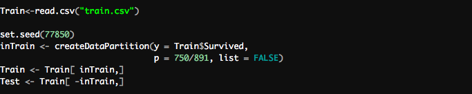
Note: Considering the small size of the original dataset, I have assigned 750 observations to the train and 141 observations to the test holdout. Further, by defining a seed value, I have ensured that the same set of random numbers are generated every time. Doing so will remove the uncertainty around the modelling results and help one assess the model’s performance accurately.
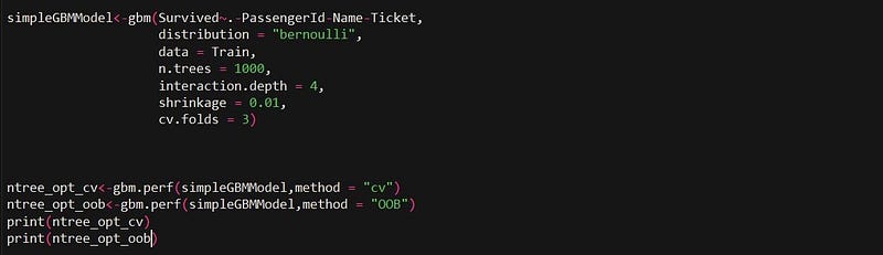
The next step is to train a gbm model using our training holdout. While all other arguments are exactly what were discussed in the previous section, there are two additional arguments that have been specified- interaction.depthand shrinkage. Interaction Depth specifies the maximum depth of each tree( i.e. highest level of variable interactions allowed while training the model). Shrinkage is considered as the learning rate. It is used for reducing, or shrinking, the impact of each additional fitted base-learner (tree). It reduces the size of incremental steps and thus penalises the importance of each consecutive iteration.
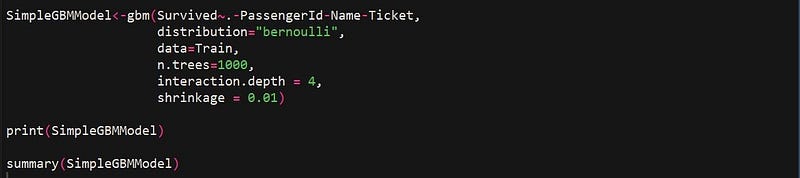
Note: Even though we are initially training our model with 1000 trees, we can prune the number of trees based on either the “Out-of-Bag or “Cross-Validation” technique to avoid overfitting. We will later see how to incorporate this in our gbm model (see the section “Tuning a gbm model and Early Stopping”)
Understanding the GBM Model Output
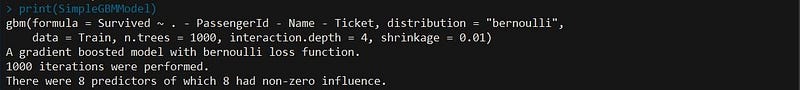
When you print a gbm model, it will remind you how many trees or iterations were used in its execution. Using its internal calculations such as Variable Importance, it will also point whether any of the predictor variables had zero influence in the model.
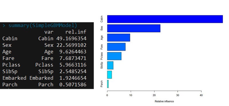
An important feature in the gbm modelling is the Variable Importance. Applying the summary function to a gbm output produces both a Variable Importance Table and a Plot of the model. This table below ranks the individual variables based on their relative influence, which is a measure indicating the relative importance of each variable in training the model. In the Titanic Model, we can see that Cabin and Sex are by far the most important variables in our gbm model.
Tuning a gbm Model and Early Stopping
Hyperparameter tuning is especially significant for gbm modelling since they are prone to overfitting. The special process of tuning the number of iterations for an algorithm such as gbm and random forest is called “Early Stopping”. Early Stopping performs model optimisation by monitoring the model’s performance on a separate test data set and stopping the training procedure once the performance on the test data stops improving beyond a certain number of iterations.
It avoids overfitting by attempting to automatically select the inflection point where performance on the test dataset starts to decrease while performance on the training dataset continues to improve as the model starts to overfit. In the context of gbm, early stopping can be based either on an out of bag sample set (“OOB”) or cross- validation (“cv”). Like mentioned above, the ideal time to stop training the model is when the validation error has decreased and started to stabilise before it starts increasing due to overfitting.
While other boosting algorithms such as “xgboost” allow the user to specify a bunch of metrics such as error and log loss, the “gbm” algorithm specifically uses the metric “error” to evaluate and measure model performance. In order to implement early stopping in “gbm”, we will first have to specify an additional argument called “c.v folds” while training our model. Secondly, the gbm package comes with a default function called gbm.perf() to determine the optimum number of iterations. The argument “method” allows the user to specify the technique used (“OOB” or “cv”) for deciding the optimum number of trees.
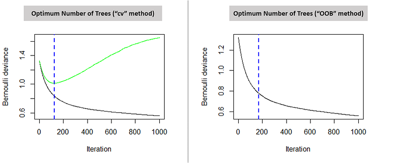
The following console screen displays the optimum number of trees as per the “OOB” and “cv” method.

Further, we will also see two plots indicating the optimum number of trees based on the respective technique used. The graph on the left indicates the error on test (green line) and train data set (black line). The blue dotted line points the optimum number of iterations. One can also clearly observe that the beyond a certain a point (169 iterations for the “cv” method), the error on the test data appears to increase because of overfitting. Hence, our model will stop the training procedure on the given optimum number of iterations.
Predictions using gbm
Finally, predict.gbm() function allows to generate the predictions out of the data. One important feature of the gbm’s predict is that the user has to specify the number of trees. Since there is no default value for “n.trees” in the predict function, it is compulsory for the modeller to specify one. Since we have figured out the optimum number of trees by performing early stopping, we will use the optimum values for specifying the “n.trees” argument. I have used the optimum solution based on the cross validation technique as cross validation usually outperforms the OOB method on large datasets. One another argument that the user can specify in the predict function is the type, which controls the type of output generated from the function. In other words, type refers to the scale on which gbm makes predictions.

Concluding and Assessing the Results:
Finally, the most important part of any modelling exercise is to assess the predictions and gauge the model’s performance. I started off by creating a confusion matrix. A really useful tool, the confusion matrix compares the model’s actual values with the predicted values. It is called a confusion matrix because it reveals how confused your model is between the two classes. The columns of the confusion matrix are the true classes while the rows of the matrix are the predicted classes. Before you make your confusion matrix, you need to “cut” your predicted probabilities at a given threshold to turn probabilities into class predictions. You can do this easily with the ifelse()function. In our example, cases with probabilities greater than 0.7 were labelled as 1 i.e likely to survive and cases with lesser probabilities were labelled as 0. Remember calling the “caret” library in order to run the confusion matrix.

Running the last line will produce our confusion matrix.
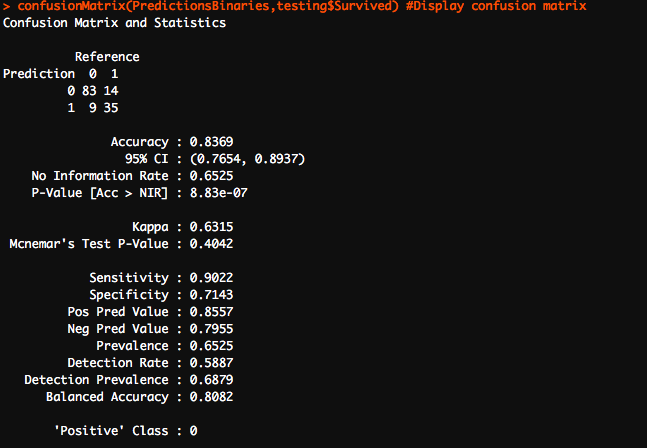
I am as delighted as you are on seeing the accuracy of our model! Diving deeper into the confusion matrix, we observe that our model perfectly predicted 118 out of 141 observations, giving us an accuracy of 83.69%. There were 23 cases that our model got wrong. These 23 cases were divided between False negatives and false positives as 9 and 14 respectively.
The ROC and the AUC: Based on the true and false positives, I produced the ROC curve and calculated our AUC value.
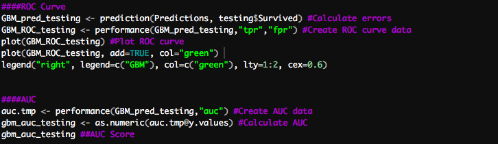
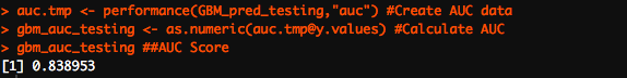
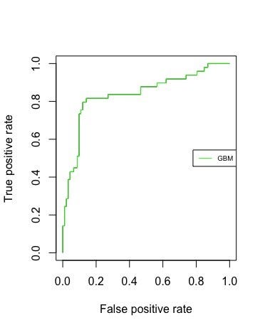
By definition, the closer the ROC curve comes to the upper left corner in the grid, the better it is. The upper left corner corresponds to a true positive rate of 1 and a false positive rate of 0. This further implies that good classifiers have bigger areas under the curves. As evident, our model has an AUC of 0.8389.
Final Remarks:
I hope that this article helped you to get a basic understanding of how the gradient boosting algorithm works. Feel free to add me on LinkedIn and I look forward to hearing your comments and feedback.In addition, I would highly recommend the following resources if you are interested in reading more about this powerful machine learning technique.
- A Gentle Introduction to the Gradient Boosting Algorithm for Machine Learning
- A Kaggle Master Explains Gradient Boosting
- Custom Loss Functions for Gradient Boosting
- Machine Learning with Tree-Based Models in R
Also, I am happy to share that my recent submission to the Titanic Kaggle Competition scored within the Top 20 percent. My best predictive model (with an accuracy of 80%) was an Ensemble of Generalized Linear Models, Gradient Boosting Machines, and Random Forest algorithms. I have uploaded my code to GitHub and it can be accessed at: https://lnkd.in/dfavxqh
Bio: Harshdeep Singh is an experienced Data Professional with a demonstrated history of working in business analysis and marketing strategy. He has successfully competed in several Kaggle Competitions (Top 20% in Titanic Survival Competition, Top 30% in House Price Prediction Challenge).
Original. Reposted with permission.
Related:
- Using Caret in R to Classify Term Deposit Subscriptions for a Bank
- Mastering The New Generation of Gradient Boosting
- Building AI to Build AI: The Project That Won the NeurIPS AutoML Challenge